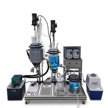
How Do Pilot Plants Expose Stokes' Law Limits In Liquid-Liquid Separation? Optimize Your Separator Design.

Simplified Stokes’ law can mislead. Unit operations pilot plants for liquid-liquid separation let you see the drag force that the textbook formula ignores. By measuring real separation rates in a horizontal separator, you immediately discover that a drag coefficient correction—based on the droplet Reynolds number—is necessary to avoid undersizing your vessel and failing to meet the target separation.

Simplified Stokes’ law (drag coefficient (C_D \approx 1.0)) assumes drag is negligible, giving a terminal settling velocity that looks fast. In a real liquid–liquid separator, drag force dominates droplet motion. Pilot plants expose this limitation, forcing you to apply a Reynolds‑number‑dependent drag coefficient before you can trust your sizing.

The Classroom Formula vs. the Real World

The Simplified Assumption We All Learned

Basic courses present Stokes’ law as ( u_t = \frac{d_m^2 (\rho_d - \rho_c) g}{18 \mu_c} ). This form assumes the drag force is small—the drag coefficient is roughly 1.0.

The equation is clean, predictable, and dangerously optimistic. It tells you droplets will settle faster than they actually will in industrial mixtures.

What You Actually Measure in a Pilot Plant

A pilot‑scale horizontal separator lets you control feed rate, measure residence time, and sample the oil‑water interface.

When you record the actual droplet settling speed, the numbers don’t match the simplified equation. The real velocity is markedly lower, and the discrepancy grows at higher fluid throughputs.

A Pilot Plant’s Honest Feedback

Visualizing Drag’s Heavy Hand

With clear vessel walls or sight glasses, you watch the droplet motion. Small droplets don’t accelerate to a swift terminal speed—they drift slowly under a continuous drag resistance.

This visual mismatch forces a mental shift: drag isn’t a minor correction; it’s the primary force balancing gravity. The simplified law’s assumption collapses.

The Reynolds Number Correction

To reconcile theory and observation, you calculate the droplet Reynolds number ((Re_p = \frac{d_m u_t \rho_c}{\mu_c})). Even at low (Re_p), (C_D) deviates from 1.0—often falling well below that value for small, slowly moving droplets.

The corrected terminal velocity must use an iterative (C_D) (e.g., from the Schiller‑Naumann correlation). The pilot plant data validates that this correction is not a mathematical luxury—it’s a design necessity.

Additional Forces the Simplified Law Ignores

In liquid–liquid extraction, the density difference is usually small and interfacial tension can be low. These physical properties, combined with the vessel geometry, create complications beyond drag.

Interfacial tension and coalescence: Low tension slows phase separation and keeps droplets suspended. The pilot plant shows that droplets take far longer to separate than a pure Stokes calculation would predict.
Axial mixing and emulsification: Backmixing and incidental emulsification from pumps or valves add turbulent dispersion. The simplified law assumes quiet, quiescent settling—a condition that rarely holds at scale.
Continuous phase velocity constraint: In a decanter, the continuous‑phase velocity through the interface must stay below the dispersed droplet settling speed. The pilot plant demonstrates that if you use the uncorrected Stokes velocity as your design limit, you will push oil‑water interfaces too high, carry over droplets, and fail to meet the water‑cut specification.

The Danger of Undersized Vessels

The Cost of Ignoring Drag

If you size a horizontal separator with the simplified law, you will choose a vessel that’s too short and too full of fluid. The actual residence time won’t allow complete phase separation, and you’ll see a rising water cut in the treated oil.

In industry, that means off‑spec product, downstream fouling, or expensive retrofits. The pilot plant makes these failures miniature and measurable, not catastrophic.

From Lab to Full‑Scale: Validation

Pilot plants provide the empirical data that simulation‑based models demand. You can collect mass balances and separation efficiencies under controlled conditions and then compare them with theoretical sizing equations that include the drag correction.

This physical verification uncovers discrepancies caused by real‑world constraints—fouling, imperfect level control, heat loss—that pure simulations might oversimplify. The result is a safer, economically viable design.

Understanding the Trade‑offs

What a Pilot Plant Cannot Tell You

A pilot‑scale separator alone won’t perfectly predict field‑scale behavior. Wall effects, mixing‑zone scaling, and surface‑active contaminant accumulation can change at full size.

Moreover, pilot‑plant experiments are time‑consuming and costly compared to a quick spreadsheet. You must use them strategically, not as a substitute for every calculation.

When Simplified Stokes is Still Useful

For early‑stage “sanity checks” or when the droplet Reynolds number is extremely low (<0.1), the simplified law gives a first estimate. It also helps students internalize the fundamental dependency on droplet size and density difference.

The key is to never let that estimate become your final sizing number. The pilot plant’s role is to teach you where the boundary of applicability lies.

Making the Right Choice for Your Separation Design

How you use a pilot plant to expose the limits of simplified Stokes depends on your primary objective.

If your primary focus is early‑stage feasibility: Run a few pilot‑scale decanting tests with your actual fluid pair. Measure the true settling velocity and back‑calculate an effective drag correction factor to feed into your sizing spreadsheet.
If your primary focus is teaching chemical engineering students: Design a pilot‑plant experiment where students compare the theoretical ( u_t ) from the simplified law with the observed interface movement. Force them to compute the droplet Reynolds number and apply the ( C_D ) correction themselves, making the drag force tangible.
If your primary focus is scaling up a critical separator: Use the pilot plant to generate a family of data points that map feed rate against water‑cut. Fit a model that includes the corrected Stokes velocity and accounts for backmixing—this becomes your validated scale‑up tool, not the textbook formula.

A pilot plant does more than prove a law is limited; it transforms a theoretical abstraction into a design responsibility you can see, measure, and finally get right.

Summary Table:

Parameter	Simplified Stokes' Law Assumption	Real-World Pilot Plant Observation
Drag Coefficient ($C_D$)	Assumed constant ($\approx 1.0$)	Varies with droplet Reynolds number ($Re_p$)
Settling Velocity	Fast, optimistic prediction	Slower due to continuous drag resistance
Additional Forces	Ignored (assumes quiescent settling)	Low interfacial tension, turbulence, backmixing
Vessel Sizing Risk	High risk of undersized decanters	Validated, accurate scale-up dimensions

Master Real-World Separation Design with LABPARK

Bridging the gap between textbook formulas and industrial reality requires hands-on validation. LABPARK provides state-of-the-art Educational and Vocational Unit Operations Pilot Plants in chemical engineering, bioprocess & biotech, and environmental & water treatment.

Specially designed for universities, research institutes, and enterprises, our pilot plants empower your students and researchers to visualize fluid dynamics, calculate precise drag corrections, and prevent costly vessel undersizing.

Take the guesswork out of chemical engineering education and scale-up. Contact us today to discuss your laboratory requirements!