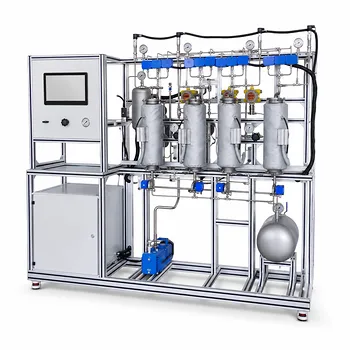
How To Determine Theoretical Stages In A Gas Absorption Pilot Plant? Graphical Method Guide

The graphical method for determining theoretical stages in a gas absorption pilot plant is a direct, visual application of mass balance and phase equilibrium principles. Students plot an operating line and an equilibrium curve on a Y-X diagram, then step off stages from the bottom composition to the target top composition. The number of steps drawn equals the number of theoretical plates required. This method bridges the fundamental theory of mass transfer with hands‑on pilot‑plant data, teaching students how real equipment performance deviates from ideal equilibrium models.

The graphical stage‑stepping technique converts steady‑state concentration measurements into a clear picture of separation difficulty and column design. Its real power in a pilot plant setting comes from the ability to calculate stage efficiency by comparing the graphical theoretical stages to the actual physical trays in the column, revealing how hydrodynamics and non‑idealities reduce real‑world performance.

Translating Pilot Plant Measurements into the Graphical Diagram

Before a single step can be drawn, the experimental data must be organized into the two lines that govern the entire separation: the equilibrium curve and the operating line.

Obtaining the Equilibrium Curve

The equilibrium relationship—the concentration of solute in the gas phase versus the liquid phase at the same temperature and pressure—is a thermodynamic property of the system. In an educational pilot plant, this is often provided from literature or can be experimentally measured in a separate equilibrium cell. For gas absorption, it is plotted as Y (gas mole ratio) against X (liquid mole ratio). The curve’s shape is critical: a highly curved equilibrium line indicates a difficult separation that will require many stages, while a shallow, near‑linear line suggests an easier task.

Plotting the Operating Line from Steady‑State Samples

The operating line represents the column’s material balance and is determined entirely from measured flow rates and compositions. Students draw liquid and gas samples at the column’s inlet and outlet under steady‑state conditions. By analyzing the solute concentration in the lean liquid inlet (top) and rich liquid outlet (bottom), along with the rich gas inlet (bottom) and lean gas outlet (top), they can calculate the coordinates of the two endpoints on the Y‑X diagram. Since the operating line is straight when the liquid and gas flow rates are constant and the solute is dilute, connecting these two points gives the full line. Its slope is the L/G ratio (liquid‑to‑gas flow ratio), a key adjustable parameter that students control by varying pump and valve settings.

Executing the McCabe‑Thiele Stepping Procedure for Absorption

Once both lines are fixed on the graph, the stage construction itself is a rote geometric exercise, yet understanding the physical meaning behind each step is what transforms the exercise from mere drawing to true engineering insight.

Starting at the Bottom and Stepping Upwards

Gas absorption columns are numbered from the bottom up. The process begins at the point representing the bottom of the column: the inlet gas composition (rich gas, Y_bottom) and the outlet liquid composition (rich liquid, X_bottom). From this starting point—often labeled point T—a horizontal line is drawn to the equilibrium curve. This horizontal movement represents the solute transfer that would occur if a theoretical stage achieved perfect equilibrium between the gas leaving that stage and the liquid leaving the same stage.

From the intersection on the equilibrium curve, a vertical line is drawn straight down to the operating line. This vertical move represents the material balance shift as the liquid drops to the next stage. The first complete triangle (horizontal then vertical) defines one theoretical stage.

Repeating Until the Target is Reached

The newly landed point on the operating line becomes the starting point for the next stage, and the same horizontal‑to‑equilibrium, vertical‑to‑operating‑line sequence is repeated. The stepping continues in a staircase fashion until a vertical drop lands on or passes the top operating point (target gas outlet composition). The total number of horizontal steps drawn is the number of theoretical stages required for the absorption task. In a perfectly designed column, this number would match the physical trays installed.

Understanding the Trade‑offs of the Graphical Method

While intuitive, the graphical technique has limitations that students must appreciate to use it wisely and to know when to switch to an analytical approach.

Sensitivity to Drawing Errors and Equilibrium Curvature

The accuracy of the stage count depends directly on the precision of the plotted lines and the careful drawing of each horizontal and vertical step. Small errors in reading compositions or in drawing the equilibrium curve can shift the stage count by half a stage or more. This is particularly problematic when the equilibrium line and operating line come close together near the top of the column, where steps become very small and hard to count. For highly curved equilibrium lines—common with concentrated solute mixtures—the stage‑by‑step drawing can become tedious and subjective, as the horizontal steps may not intersect a cleanly defined curve.

When the Analytical Kremser Method is Superior

For dilute systems where the equilibrium line is linear (Y* = mX), the graphical method is often set aside in favor of the Kremser equation. This analytical approach calculates the number of stages N directly from the unabsorbed solute fraction Φ_A and the absorption factor A (L/mG). The Kremser method eliminates drawing errors and provides a precise, repeatable result. In a pilot plant experiment, students can measure inlet and outlet gas concentrations, compute Φ_A, and then solve N = ln[((1 - 1/A)/Φ_A) + 1/A] / ln(A). Comparing the graphical stage count with the Kremser result for a linear system is an excellent way to quantify the graphical method’s inherent uncertainty and to reinforce when each tool is appropriate.

The Missing Link: From Theoretical to Actual Stages

A graph on paper always assumes 100% stage efficiency. Real trays do not achieve equilibrium; liquid entrainment, weeping, and imperfect mixing reduce separation per tray. The graphical method gives the idealized, thermodynamic limit. The pilot plant’s true value emerges when students count the actual physical trays in the column (say, 10 real trays) but calculate 8 theoretical stages. The ratio (theoretical / actual) is the overall column efficiency. This efficiency number encapsulates all the non‑idealities that separate textbook theory from industrial reality.

Calculating Stage Efficiency from the Pilot Plant Data

The ultimate purpose of the pilot plant exercise is not merely to produce a number of stages, but to characterize the equipment itself.

Comparing Graphical Stages with Physical Hardware

After running the column at steady state, students have all the composition endpoints needed for the graphical construction. They count the physical trays (or packed height equivalent) inside the pilot plant. By dividing the number of graphical theoretical stages by the number of real trays, they obtain the overall tray efficiency. For example, 6 theoretical stages from the graph paired with a 10‑tray column yields a 60% efficiency. This metric immediately tells the engineer how effectively the internals are performing and can be used to diagnose flooding, weeping, or maldistribution if the efficiency is unexpectedly low.

Verifying Operating Window Boundaries

A reliable stage efficiency measurement is only valid if the column was operating within its safe hydrodynamic window. Flooding, weeping, or insufficient liquid holdup all degrade contact and lower the apparent stage efficiency. Students should cross‑check their L/G ratio and flow rates against the column’s performance diagram, staying clear of entrainment flooding, weeping, and downcomer backup limits. If the pilot plant was operated with a gas velocity too close to the weeping line, the measured efficiency will be artificially low, and the graphical stages will seem further from reality. This teaches the critical lesson that theoretical models are only as good as the experimental conditions they test.

Making the Right Choice for Your Absorption Experiment

The graphical method remains a foundational teaching tool, but its application should be deliberate. Use these goal‑oriented guidelines to align your approach with what you need to learn.

If your primary focus is to visualize the separation process and build intuition: The graphical Y‑X stepping method is irreplaceable. Draw the diagram carefully, count the steps, and discuss each triangle’s meaning with your team to cement your understanding of stage‑wise contact.
If your primary focus is to obtain a rapid, precise stage count for a dilute, linear‑equilibrium system: Use the analytical Kremser equation. The results will be free from graphical errors, and you can then compare this mathematical ideal against your pilot plant’s actual performance.
If your primary focus is to evaluate the pilot plant’s hardware performance: Run the graphical method, count the physical trays, and compute the overall column efficiency. This efficiency figure is your most valuable deliverable, as it quantifies the gap between theory and the real equipment on your bench.

Theoretical stages are not just a number to be circled on a lab report—they are the lens through which you see the invisible mass transfer happening inside your column, and mastering the graphical method is the first step toward optimizing any gas separation process.

Summary Table:

Method	Best Used For	Key Inputs	Main Advantage	Limitations
Graphical Method	Visualizing stage-wise separation & curved equilibrium lines	Operating line endpoints (L/G ratio) & Equilibrium curve	Provides visual intuition & identifies stage efficiency	Prone to drawing errors, especially in pinched regions
Analytical (Kremser)	Dilute, linear-equilibrium systems ($Y^* = mX$)	Absorption factor ($A$) & unabsorbed solute fraction	Fast, precise, and free of human drawing error	Only applicable to straight equilibrium lines

Enhance Your Engineering Lab with LABPARK Pilot Plants

To truly understand chemical separation processes, students need high-quality, real-world equipment. LABPARK designs and supplies state-of-the-art Educational and Vocational Unit Operations Pilot Plants in chemical engineering, bioprocess & biotech, and environmental & water treatment.

Our systems are tailored for universities, research institutes, and enterprises to bridge the gap between textbook formulas and physical plant operations.

Ready to upgrade your lab's training capabilities? Contact LABPARK today to request a quote or discuss a custom pilot plant configuration for your program!