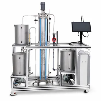
Why Do Multicapacity Process Units, Such As Multi-Stage Liquid Systems Or Distillation Column Pilot Plants, Display An S-Shaped Step Response? Explained

Multicapacity process units display an S-shaped step response because several storage elements respond sequentially rather than simultaneously. In a multi-tank system, each tank must accumulate material before significantly changing the next tank’s level or flow. In a distillation column, each tray or section must exchange mass and energy with neighboring stages, creating a series of interacting dynamic lags.

An S-shaped response is the visible result of multiple first-order lags in series: the process initially changes slowly, responds most rapidly in the middle of the transient, and then gradually approaches its final steady state.

Why the Response Begins Slowly

The First Capacity Responds Before the Others

A step input changes the first capacity immediately, but downstream capacities initially remain close to their original conditions. The first stage must build up enough material or thermal energy before it can produce a substantial change in the next stage.

This creates an initial period of sluggish response. It resembles dead time, but it is usually caused by distributed storage and transfer dynamics rather than by a true transport delay.

Each Stage Adds Transfer Lag

After the first stage begins responding, the next stage responds to the changing output from the first. The same process repeats through the remaining capacities.

Because each stage reacts to a changing, delayed signal from the previous stage, the total response is slower and smoother than the response of any single capacity.

Why the Curve Becomes Steeper

Delayed Effects Accumulate

Once the disturbance has propagated through several stages, multiple capacities are changing at the same time. The process output then responds more rapidly, producing the steep central portion of the S-shaped curve.

The response rate is therefore not constant. It starts near zero, increases as the disturbance moves through the system, and later decreases as the system approaches equilibrium.

Cascaded Lags Produce the S Shape

For a sequence of identical first-order lags, the transfer function can be represented approximately as:

[ G(s)=\frac{K}{(\tau s+1)^n} ]

where (K) is the overall process gain, (\tau) is the characteristic time constant of each stage, and (n) is the number of capacities or effective stages.

With two or more lags, the output does not immediately develop its full slope. The combined response has a gradual beginning, a faster middle region, and a gradual final approach, which creates the characteristic S shape.

How the Response Finishes

The Rate Falls Near Steady State

As the downstream capacities approach their new operating conditions, the difference driving further change becomes smaller. Material or energy continues to redistribute, but the output changes progressively less with time.

This produces the flattening upper portion of the response curve.

More Stages Increase Sluggishness

Adding capacities in series generally increases the delay before the output responds substantially. It also spreads the transient over a longer interval and makes the response more distributed.

This is why a multistage column or a long sequence of connected tanks often appears slower than a single tank with a comparable overall gain.

What This Means for Distillation Column Pilot Plants

Trays Behave as Interacting Capacities

Each distillation tray can store liquid and vapor holdup and participate in mass and energy transfer. A change introduced at one location must propagate through neighboring trays before the effect becomes prominent at the measured output.

The column therefore behaves like a system with multiple interacting lags rather than a single lumped storage element.

Measurements Reflect the Selected Location

The observed S shape depends on where the input is applied and where the output is measured. A disturbance measured near its point of introduction may respond relatively quickly, while a measurement at the opposite end of the column may show a longer and more pronounced lag.

Column operating conditions also affect the effective dynamics because holdup, flow rates, phase equilibrium, and tray efficiency can change.

Why Engineers Use Dead-Time Approximations

Distributed Lag Can Resemble Dead Time

Although the response begins changing immediately in an ideal mathematical model of cascaded lags, the initial change may be too small to detect in practice. The measured curve can therefore look as though a pure delay occurred before the process started responding.

Engineers often approximate the behavior using a first-order-plus-dead-time model:

[ G(s)\approx\frac{K e^{-\theta s}}{\tau s+1} ]

where (\theta) represents apparent dead time and (\tau) represents the remaining dominant lag.

The Approximation Supports Controller Design

This simplified model is useful for estimating process gain, apparent delay, and response speed from a pilot-plant step test. Those estimates can then support initial proportional-integral-derivative controller tuning.

The approximation is a modeling convenience, not a claim that all of the delay is a literal transport delay.

Understanding the Trade-offs

The Model Is Simpler Than the Real Process

Representing many capacities as one apparent lag and one dead time makes analysis and controller tuning practical. However, it can hide the individual stage dynamics and may become inaccurate when the process operates far from the test condition.

More Capacity Does Not Always Mean More Pure Delay

A larger number of stages usually increases the apparent sluggishness, but the exact curve depends on the time constants, gains, and interactions of the stages. Unequal time constants can produce behavior that differs substantially from a simple chain of identical lags.

Aggressive Control Can Amplify Process Limitations

A controller tuned as though the process were fast may overreact to a slow multicapacity unit. This can cause overshoot, oscillation, or actuator saturation before the full effect of a control action becomes visible.

Nonlinear Effects May Distort the S Shape

Real liquid and distillation systems may exhibit nonlinear flow, phase-equilibrium, holdup, and heat-transfer behavior. A step response taken at one operating point should therefore be treated as a local dynamic description rather than a universal model.

Making the Right Choice for Your Goal

The most useful interpretation depends on what you need to accomplish with the pilot plant.

If your primary focus is understanding the transient: Recognize the S shape as the combined effect of sequential mass or energy storage and transfer through multiple capacities.
If your primary focus is identifying a process model: Fit the response using a cascaded-lag model or a first-order-plus-dead-time approximation, while checking whether the approximation captures the measured dynamics.
If your primary focus is controller tuning: Account for the apparent delay and sluggishness before selecting aggressive tuning parameters.
If your primary focus is comparing plant configurations: Expect additional stages or longer series connections to increase propagation lag and extend the overall settling time.

The S-shaped response is therefore a practical signature of distributed storage: the process reacts progressively as a disturbance travels through its connected capacities.

Summary Table:

Key aspect	Explanation	Engineering implication
Initial response	Sequential storage and transfer create a slow beginning that can resemble dead time.	Avoid assuming the process has a true transport delay.
Steep middle region	Several capacities respond simultaneously as the disturbance propagates.	The process response rate increases during the transient.
Final response	Driving forces decrease as the system approaches equilibrium.	The output gradually settles at its new steady state.
Distillation columns	Trays store liquid and vapor while exchanging mass and energy.	Measurement location and tray conditions affect the observed dynamics.
Process modeling	Cascaded-lag or first-order-plus-dead-time models approximate the response.	Use step-test data to estimate gain, delay, and time constants.
Control considerations	Sluggish dynamics can make aggressive tuning cause overshoot or oscillation.	Account for apparent delay and settling time during controller design.

Need to study or control multistage process dynamics? Contact LABPARK to discuss an Educational or Vocational Unit Operations Pilot Plant tailored to your objectives. LABPARK provides pilot plants for chemical engineering, bioprocess and biotech, and environmental and water treatment applications. Universities and research institutes can use our systems for hands-on teaching, process modeling, step-response testing, and controller tuning. Enterprises can evaluate process behavior, train operators, and validate control strategies with practical laboratory-scale equipment. Tell us your process, number of stages, measurement requirements, and training or research goals, and our team will help identify a suitable configuration.