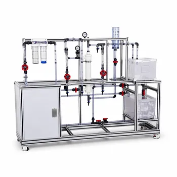
The transverse pressure gradient is assumed to be zero because a high-Reynolds-number boundary layer is very thin compared with the equipment’s characteristic length. In the wall-normal direction, the pressure variation across this thin region is negligible at leading order, so the boundary-layer momentum equation reduces to (\partial p/\partial y \approx 0). The pressure within the boundary layer is therefore set by the outer, essentially inviscid flow.

In boundary-layer analysis, pressure changes mainly along the surface, not across the boundary-layer thickness. This lets engineers use the outer-flow pressure distribution to analyze the boundary layer, including its stability, separation, and transition behavior.

Why the Boundary Layer Approximation Works

The boundary layer has two very different length scales

A boundary layer has a streamwise length scale (L) and a much smaller wall-normal thickness (\delta), where

[ \delta \ll L. ]

The velocity changes rapidly across (\delta), from zero at the wall to nearly the external-flow velocity at the boundary-layer edge. Pressure, however, does not undergo a similarly large change across this small distance.

In pilot plant equipment, this applies to thin flow regions near walls in channels, pipes, heat exchangers, diffusers, and contoured surfaces, provided the flow has a sufficiently high Reynolds number and the boundary-layer assumptions remain valid.

The wall-normal momentum equation simplifies

For steady two-dimensional flow, the wall-normal Navier-Stokes equation contains terms such as

[ \rho\left(u\frac{\partial v}{\partial x} +v\frac{\partial v}{\partial y}\right)

-\frac{\partial p}{\partial y} +\text{viscous terms}. ]

Boundary-layer scaling shows that the inertial and viscous terms in the (y)-direction are smaller than the dominant streamwise terms. To leading order, the equation becomes

[ \frac{\partial p}{\partial y}=0. ]

This does not mean that pressure is constant everywhere. It means that pressure is approximately constant across the boundary layer at a given streamwise location.

The pressure still changes along the wall

The streamwise pressure gradient generally remains important:

[ \frac{\partial p}{\partial x}\neq 0. ]

The external flow may accelerate or decelerate as it moves downstream. This produces a favorable pressure gradient when pressure decreases in the flow direction and an adverse pressure gradient when pressure increases.

Thus, the approximation is better expressed as

[ p(x,y)\approx p_e(x), ]

where (p_e(x)) is the pressure at the boundary-layer edge.

What Sets the Pressure Inside the Boundary Layer?

The outer flow imposes the pressure field

Outside the boundary layer, viscous effects are relatively weak, so the outer flow can often be treated as inviscid. Its pressure distribution is determined by the equipment geometry and the resulting mainstream velocity field.

Because the pressure is nearly uniform in the wall-normal direction,

[ p_{\text{boundary layer}}(x,y) \approx p_e(x). ]

The boundary layer therefore responds to the pressure distribution created by the outer flow rather than generating an independent wall-normal pressure field.

The pressure at the wall follows the outer pressure

At the solid wall, the leading-order boundary-layer result gives

[ p_w(x)\approx p_e(x). ]

This is why wall static-pressure measurements can often represent the pressure distribution imposed on the boundary layer. In pilot plant experiments, pressure taps along a wall can therefore be used to evaluate the streamwise pressure gradient affecting near-wall flow.

This interpretation applies when the pressure tap is properly designed and the flow remains within the regime where boundary-layer theory is appropriate.

Why the Pressure Variation Across the Layer Is Small

Scaling explains the small transverse change

Let (x) scale with (L), (y) scale with (\delta), and define the small parameter

[ \epsilon=\frac{\delta}{L}. ]

For a thin boundary layer, (\epsilon\ll 1). The rapid variation in velocity across (y) does not imply a comparable pressure variation because the wall-normal momentum balance is smaller by powers of this thinness parameter.

The pressure difference between the wall and the boundary-layer edge is therefore a higher-order effect. In common nondimensional formulations, it is of order (O(\epsilon^2)), which is related to (O(Re^{-1})) for standard boundary-layer scaling.

Thinness is the essential assumption

The approximation depends on the boundary layer being thin. Increasing Reynolds number generally reduces the relative boundary-layer thickness, making the assumption more accurate.

Conversely, the approximation becomes less reliable when the boundary layer is no longer thin compared with the equipment geometry or when strong three-dimensional and separated-flow effects dominate.

Why the Streamwise Pressure Gradient Matters

Favorable pressure gradients tend to stabilize the layer

A favorable pressure gradient means

[ \frac{\partial p_e}{\partial x}<0 ]

in the direction of the external flow. The outer flow accelerates, and the boundary-layer velocity profile generally becomes fuller.

This tends to reduce the susceptibility of a laminar boundary layer to instability and can delay transition or separation.

Adverse pressure gradients promote separation

An adverse pressure gradient means

[ \frac{\partial p_e}{\partial x}>0. ]

The outer flow decelerates, while fluid near the wall has already lost kinetic energy through viscous effects. The near-wall fluid may then be unable to overcome the increasing pressure.

At separation, the wall shear stress approaches zero:

[ \tau_w

\mu\left.\frac{\partial u}{\partial y}\right|_{y=0} =0. ]

With a stronger adverse pressure gradient, the near-wall flow can reverse direction. The transverse pressure gradient is still approximately zero within the boundary-layer approximation, but the streamwise pressure gradient controls the separation process.

How This Applies to Pilot Plant Training Systems

Pressure measurements can be interpreted more simply

Because the pressure is approximately uniform through the boundary-layer thickness, the external pressure distribution can be applied directly when analyzing velocity profiles, wall shear, and boundary-layer growth.

This reduces the need to measure pressure at multiple wall-normal positions within the thin layer. Measurements along the wall are usually more useful for identifying the streamwise pressure gradient.

Geometry determines the imposed pressure distribution

A converging passage, contoured surface, diffuser, bend, or heat-exchanger channel can create different external pressure distributions.

The boundary layer responds to those distributions, so changes in geometry can be connected experimentally to acceleration, deceleration, transition, separation, pressure loss, and heat or mass transfer performance.

The approximation supports teaching and diagnosis

In a pilot plant, students can treat the outer pressure field as known and then examine how the boundary layer responds. This separates two related problems: determining the mainstream pressure distribution and determining the near-wall velocity and shear response.

That distinction is central to interpreting boundary-layer experiments.

Understanding the Trade-offs

Zero does not mean exactly zero

The statement

[ \frac{\partial p}{\partial y}=0 ]

is a leading-order approximation. Small wall-normal pressure variations can exist, particularly when the boundary layer is thick, the flow is strongly curved, or the flow is separated and highly unsteady.

The correct physical statement is that the transverse pressure gradient is negligible relative to the dominant terms under boundary-layer scaling.

The approximation does not remove pressure effects

Pressure remains a major influence on the boundary layer through (\partial p_e/\partial x). Assuming (\partial p/\partial y\approx 0) does not mean that pressure can be ignored.

It means that pressure is transmitted across the boundary layer from the outer flow, while its important variation occurs along the surface.

Separation weakens simple boundary-layer assumptions

Near separation, velocity gradients, reverse flow, turbulence, and unsteadiness become increasingly important. After large-scale detachment, the flow may no longer behave as a thin attached boundary layer.

Pilot plant results near recirculation zones, abrupt expansions, strong bends, or diffuser stall should therefore be interpreted with caution.

Three-dimensional effects may matter

The simple form (\partial p/\partial y=0) is most directly associated with two-dimensional or gently varying boundary-layer flow. Strong curvature, secondary flows, rotation, swirl, and cross-stream motion can require more complete analysis.

Making the Right Choice for Your Goal

The approximation is useful when the experiment satisfies the assumptions behind thin, high-Reynolds-number boundary-layer theory.

If your primary focus is boundary-layer velocity profiles: Use the measured or calculated outer pressure (p_e(x)) as the pressure throughout the boundary layer at each streamwise position.
If your primary focus is transition or stability: Concentrate on the streamwise pressure gradient, especially the locations of favorable and adverse pressure gradients.
If your primary focus is separation: Monitor the adverse pressure gradient, boundary-layer profile, and wall shear stress rather than looking for a significant transverse pressure variation.
If your primary focus is pressure instrumentation: Wall static-pressure taps can usually represent the outer pressure imposed on an attached thin boundary layer, subject to proper tap placement and flow conditions.

The transverse pressure gradient can be neglected because thin-boundary-layer scaling makes its effect higher order, while the outer-flow pressure variation along the wall remains the quantity that governs the boundary layer’s behavior.

Summary Table:

Key concept	Practical meaning
Thin-layer assumption	Boundary-layer thickness is much smaller than the equipment length scale.
Transverse pressure gradient	Approximately zero: `∂p/∂y ≈ 0` across the boundary layer.
Pressure distribution	Pressure inside the layer follows the outer-flow pressure, `p(x,y) ≈ p_e(x)`.
Streamwise pressure gradient	Controls acceleration, deceleration, transition, and separation.
Favorable gradient	Can stabilize the boundary layer and delay separation.
Adverse gradient	Can reduce wall shear and cause flow separation.
Main limitations	Thick, separated, strongly curved, three-dimensional, or unsteady flows may require advanced analysis.
Pilot plant application	Wall pressure taps can help evaluate the pressure gradient affecting near-wall flow.

Need practical training equipment for boundary-layer and fluid-flow education? Contact LABPARK to discuss Educational and Vocational Unit Operations Pilot Plants designed for universities, research institutes, and enterprises. LABPARK provides configurable systems for chemical engineering, bioprocess and biotechnology, and environmental and water treatment training. Our pilot plants help learners and engineers connect pressure measurements, velocity profiles, wall shear, transition, separation, and process performance through hands-on experiments. Tell us your teaching, research, or industrial training goals, and LABPARK can help you select and configure a reliable pilot plant for your laboratory.