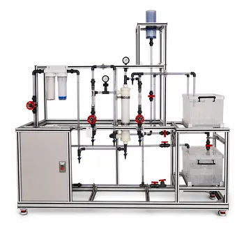
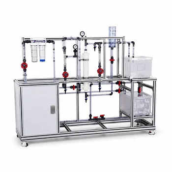
What Parameters Can Researchers And Students Optimize When Operating An Md Pilot Plant? Maximize Desalination Efficiency

The deceptively simple levers of temperature, flow, and salinity hold the key to unlocking your MD pilot plant’s full potential. Unlike pressure-driven membranes, the performance of membrane distillation hinges entirely on the vapor pressure gradient you create—and you control that by fine-tuning the feed temperature, coolant temperature, flow rates, and feed salinity. These four operational parameters directly dictate water vapor flux, thermal efficiency, and fouling behavior, making them the primary variables every researcher or student must master when running a thermal desalination study.

A membrane distillation pilot plant is not just a black box to produce pure water—it’s a dynamic system where the interplay of heat transfer, mass transfer, and membrane integrity reveals the true cost of desalination. By systematically optimizing temperature, flow, and feed chemistry, you can shift the process from a simple demonstration into a precise platform for studying solar‑driven performance, scaling resistance, and industrial waste‑heat utilization.

How Feed and Coolant Temperatures Control the Driving Force

The temperature difference across the membrane is the engine of MD. In a Direct Contact Membrane Distillation (DCMD) configuration, hot feed flows on one side while a cold coolant stream flows on the other, creating a partial pressure difference that drives water vapor through the pores. Raising the feed temperature increases the vapor pressure on the hot side exponentially, while lowering the coolant temperature suppresses it on the permeate side. This gradient is what you are truly optimizing.

The Feed Temperature Sweet Spot

You will see flux rise sharply as the feed temperature climbs. This is because the relationship between temperature and vapor pressure is non‑linear—small increases near 70–80 °C yield disproportionately higher permeate output. However, you must balance this against thermal energy input and the risk of damaging heat‑sensitive components or inducing premature scaling. In a pilot plant, operating close to the membrane’s thermal stability limit (often 80–90 °C for polymeric materials) lets you observe the transition from purely thermal efficiency to scaling‑dominated performance decay.

Coolant Temperature and the Invisible Thief of Efficiency

A low coolant temperature sharpens the driving force, but it also accelerates conductive heat loss through the membrane matrix. This conductive loss acts like a thief, stealing heat that should have been used for vaporization. You will measure this directly through the thermal efficiency of the system. By systematically varying the coolant temperature while keeping the feed temperature constant, you can pinpoint the exact point where flux gains are outweighed by drastically reduced energy efficiency—a core lesson in sustainable thermal desalination.

Flow Rates: The Art of Managing Boundary Layers

The bulk temperatures you set on the control panel are not the temperatures that really matter. Right next to the membrane surface, thin boundary layers of cooler feed and warmer permeate form, starving the system of its driving force. Flow rate is your tool to fight back.

Increasing Flow to Reclaim Temperature Polarization

Higher flow velocities increase turbulence, thinning these stagnant layers and reducing temperature polarization. You will see a tangible jump in flux simply by increasing the cross‑flow velocity, even with identical bulk temperatures. In pilot‑scale studies, you can plot the mass transfer coefficient against flow rate to identify the transition from laminar to turbulent regimes—a vital hands‑on experience that connects textbook heat and mass transfer equations to real‑world observation.

The Hidden Energy Cost of High Flow

Pumping energy is not free. While high flow rates boost flux, they also raise the feed‑side pressure drop and the auxiliary electricity consumption of your pumps. In your pilot plant, you will be able to trace the point of diminishing returns: the moment the incremental gain in water production is smaller than the extra energy you spend moving the fluid. This trade‑off is crucial for comparing MD to other desalination technologies that rely on electrical power.

Feed Salinity: From Salt Rejection to Scaling Onset

One of MD’s signature advantages is its near‑complete rejection of non‑volatile solutes. You can raise the feed salinity far beyond what reverse osmosis can handle and still produce ultra‑pure water. But salinity is not a passive variable—it shapes both the thermodynamic driving force and the timeline of membrane failure.

How Salt Lowers Vapor Pressure

Dissolved salts depress the vapor pressure of water according to Raoult’s law. The hotter your feed, the more pronounced this effect becomes. By experimenting with brines of 35 g/L (seawater) up to 150 g/L or more, you will directly measure a slight but measurable flux reduction. This data is invaluable for validating modeling approaches that aim to simulate MD performance in zero‑liquid‑discharge (ZLD) scenarios where salinity continuously rises.

The Real Enemy: Sparingly Soluble Salts

Sodium chloride is relatively forgiving. The true operational threat comes from sparingly soluble species like calcium sulfate (gypsum) or calcium carbonate. When these salts saturate near the membrane surface due to water removal and precipitation, scaling begins. This scaling clogs pores and can eventually force the hydrophobic membrane to wet, introducing a direct liquid path and ruining permeate quality. In your pilot plant, deliberately dosing the feed with these scalants lets you study induction times, cleaning cycles, and the role of feed pre‑treatment—moving from a simple water quality test to a serious investigation of membrane durability.

Configuration Choice: DCMD and the Path to Customization

The primary reference configuration is Direct Contact Membrane Distillation, but your pilot plant likely allows you to explore other setups such as air‑gap (AGMD) or vacuum‑assisted (VMD) modes. This choice is an optimization parameter in itself.

When to Stay with DCMD

DCMD offers the simplest construction and the highest permeation rates, making it ideal for demonstrating the fundamental transport mechanism. It works best when you have a clean, warm feed and an available cold water source. However, the direct contact creates high conductive heat loss, so it serves as your baseline for comparing thermal efficiency improvements.

Exploring Sweep Gas or Vacuum for Energy Efficiency

Switching to a vacuum on the permeate side (VMD) can drastically increase the driving force at lower feed temperatures—perfect for simulating solar‑thermal applications where the heat source might not reach 90 °C. An air gap (AGMD) inserts a stagnant layer of air between the membrane and a condensing surface, virtually eliminating conductive losses but also lowering flux. Running these configurations side‑by‑side teaches the practical truth that no single MD design is universally optimal; the choice depends on the energy source and the end‑goal.

Understanding the Trade-offs

Optimizing an MD system is not a race to maximum flux. You must weigh several competing factors that are as instructive as the mass transfer data itself.

Flux versus Thermal Efficiency

Pushing feed temperature to the max increases production but often drags thermal efficiency below 30–40 %. You will discover that the most energy‑efficient operating point often sits at a surprisingly modest temperature gradient, especially when waste heat or solar collectors are your heat source.

High Flow versus Pumping Costs

Aggressive cross‑flow reduces polarization but turns your pilot plant into a significant electrical consumer. In solar‑driven projects, every watt of pumping power competes with the solar energy you could be using directly for heating. The optimum always lies at the intersection of hydraulic behavior and the available energy budget.

Membrane Longevity versus Performance

A highly porous, thin membrane will give you sky‑high initial flux, but it may wet or scale faster under aggressive conditions. You trade short‑term experimental throughput for the long‑term data needed to assess cleaning‑in‑place protocols and membrane replacement cycles—essential knowledge for any real‑world desalination engineer.

How to Apply This to Your Project

Your optimization sequence should match your specific learning or research objective. Use this roadmap to design your experimental plan.

If your primary focus is comparing solar‑thermal MD configurations: Fix the feed and coolant loop to simulate the specific temperatures of a solar collector outlet (e.g., 60–80 °C) and then vary flow rate and membrane type to find the most stable, high‑flux combination. Evaluate thermal efficiency under these moderate‑temperature constraints because that is what a real solar system will deliver.
If your primary focus is studying scaling and wetting phenomena: Keep the temperature and flow constant at a moderate setpoint, then systematically increase the feed salinity with sparingly soluble salts. Monitor flux decline and conductivity breakthrough to map the failure point. Use these experiments to test anti‑scalant doses or intermittent flushing strategies, not to maximize water output.
If your primary focus is teaching the fundamentals of heat and mass transfer: Start with pure water and a fixed salinity, then step‑change each parameter independently—feed temperature, coolant temperature, and flow rate—while calculating the mass transfer coefficient. Plot the data against model predictions to make temperature and concentration polarization tangible. Add salt later only after the ideal behavior is understood.
If your primary focus is evaluating industrial wastewater ZLD potential: Run with a high‑salinity feed (>100 g/L) and prioritize stable operation over high flux. Monitor thermal energy consumption per unit of water produced, and compare DCMD with AGMD to find the lowest energy penalty for treating brine to near‑saturation.

Every parameter you adjust tells a story about how heat, mass, and momentum intertwine inside a hydrophobic pore. Master the interplay of temperature, flow, and chemistry in your pilot plant, and you will not just be collecting data—you will be charting the real path toward low‑energy, thermally driven desalination.

Summary Table:

Parameter	Impact on Performance	Key Optimization Goal
Temperature	Drives vapor pressure gradient	Maximize flux while minimizing conductive heat loss
Flow Rates	Reduces temperature polarization	Balance flux gains against pumping energy costs
Feed Salinity	Dictates vapor pressure & scaling	Assess membrane scaling limits & ZLD potential
Configuration	Controls heat efficiency & driving force	Align MD mode (DCMD/VMD/AGMD) with heat sources

Unlock the full potential of your research and training programs with LABPARK. We provide premium Educational and Vocational Unit Operations Pilot Plants in chemical engineering, bioprocess & biotech, and environmental & water treatment for universities, research institutes, and enterprises. Our systems enable students and researchers to easily experiment with and optimize critical parameters like temperature, flow, and salinity. Contact us today to discover how our pilot plants can enhance your academic and research outcomes!