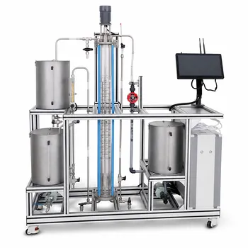
What Numerical Solution Techniques Are Required For Complex Process Dynamics? Choose Robust Methods For Pilot Units

The required numerical techniques are iterative nonlinear algebraic solvers and time-integration algorithms. A multi-tray distillation column or reactor pilot unit is represented by coupled material and energy balances, equilibrium relations, and flow equations. Because these relationships are nonlinear and tightly coupled, simulation typically requires methods such as Newton-Raphson or successive substitution for algebraic equations and Runge-Kutta, predictor-corrector, or implicit stiff ODE solvers for dynamic equations.

The central challenge is solving a coupled nonlinear differential-algebraic system. Algebraic solvers determine instantaneous equilibrium and flow variables, while integration algorithms advance tray, reactor, temperature, concentration, and pressure states through time.

Why These Pilot-Unit Models Are Numerically Difficult

Coupled Material and Energy Balances

Each tray or reactor volume has dynamic accumulation terms for components, total mass, and often energy. These balances produce many first-order nonlinear differential equations whose solutions depend on temperatures, compositions, phase flows, reaction rates, and operating conditions.

A ten-tray binary distillation model can already contain 24 nonlinear differential equations and 21 nonlinear algebraic equations. Adding more trays, components, reactions, or energy balances increases both the number and coupling of unknowns.

Nonlinear Equilibrium and Flow Relationships

Distillation models require vapor-liquid equilibrium relationships, tray compositions, vapor and liquid flow rates, condenser behavior, and reboiler behavior. Reactor models add nonlinear reaction kinetics, heat-transfer relationships, and possibly pressure-dependent rates.

These relationships cannot generally be isolated and solved analytically. The simulator must repeatedly estimate the unknown variables and reduce the residual errors until the equations are satisfied.

Differential-Algebraic Structure

The combined model is often better understood as a differential-algebraic equation system, or DAE, rather than as a set of independent ODEs. Differential variables include tray holdups, reactor concentrations, and temperatures; algebraic variables include equilibrium compositions, flow rates, and instantaneous constraints.

This distinction matters because treating every variable as an independent dynamic state can create numerical instability, redundant equations, or physically inconsistent results.

Solving the Algebraic Equations

Newton-Raphson Iteration

The Newton-Raphson method is a primary technique for solving the nonlinear algebraic equations at steady state or at each dynamic time step. It uses the residual equations and their Jacobian to calculate a correction to the current estimate.

For a vector of unknowns (z), the method solves an update of the form:

[ J(z_k)\Delta z=-R(z_k) ]

where (R(z_k)) is the residual vector and (J(z_k)) is its Jacobian. The estimate is then updated as (z_{k+1}=z_k+\Delta z).

Newton-Raphson can converge rapidly when the initial estimate is reasonable and the Jacobian is well behaved. It is particularly useful for tightly coupled tray compositions, temperatures, flow rates, and reactor states.

Successive Substitution

Successive substitution, also called fixed-point iteration, repeatedly evaluates the model equations using the latest available estimates. It is simpler to implement than Newton-Raphson and may be adequate for mildly nonlinear relationships.

Its main limitation is convergence speed. Strongly interacting stages, high reflux conditions, severe reaction nonlinearities, or poor initial estimates can cause slow convergence or divergence.

Interval Halving

Interval halving, or bisection, is a robust method for scalar nonlinear equations when a valid sign-changing interval is known. It is slower than Newton-Raphson but less sensitive to the initial guess.

It is useful for individual bounded calculations, such as locating a temperature, pressure, or flow value that satisfies a residual equation. It is generally not the main solver for a large multivariable column model.

Jacobians, Scaling, and Initial Guesses

The quality of the algebraic solution depends heavily on the Jacobian, variable scaling, and initial conditions. Composition, temperature, flow, and holdup variables can have very different magnitudes, so poor scaling can make an otherwise valid algorithm appear unstable.

A practical simulator should enforce physical bounds, use consistent initial conditions, and provide good steady-state guesses before starting a transient calculation.

Integrating the Dynamic Equations

Explicit Euler and Higher-Order Methods

An explicit method calculates the next state directly from the current state. Euler's method is simple, but its accuracy is limited and it may require very small time steps.

Higher-order explicit methods, especially fourth-order Runge-Kutta, provide better accuracy for smooth, non-stiff dynamics. They are useful for educational models and pilot-unit simulations where the time scales are not extremely different.

Predictor-Corrector Algorithms

A predictor-corrector method first predicts the future state and then corrects that prediction using updated derivative information. This can improve accuracy without requiring the full cost of a high-order method at every step.

Implicit predictor-corrector methods are more suitable when the calculated state strongly affects the derivatives, as occurs with coupled heat and mass transfer or reaction kinetics.

Implicit Methods for Stiff Dynamics

Distillation columns and reactors often contain several time scales. Tray holdup dynamics, vapor-liquid equilibrium, heat transfer, and fast reactions may respond at very different rates. This creates stiffness, where an explicit method must use an impractically small time step to remain stable.

For stiff systems, use an implicit solver, such as a backward differentiation formula or an implicit Runge-Kutta method. Each implicit time step requires solving a nonlinear algebraic system, commonly with Newton-Raphson iteration.

Adaptive Time Stepping

The solver should adjust the time step according to estimated integration error and system behavior. Small steps are needed during startup, feed changes, control actions, and sharp reaction or temperature transients; larger steps are efficient during slowly changing operation.

Adaptive stepping improves efficiency while preserving accuracy. It also helps detect numerical problems that a fixed, overly large time step might conceal.

How the Techniques Work Together

Steady-State Initialization

A robust workflow first solves the steady-state material, energy, equilibrium, and flow equations. The resulting solution supplies physically consistent initial conditions for the dynamic simulation.

Starting from arbitrary tray compositions or reactor concentrations can force the transient solver to spend excessive effort recovering feasibility or can cause the nonlinear iterations to fail.

Nonlinear Solution at Each Time Step

At each time step, the integration algorithm evaluates the dynamic balances. If the model includes algebraic constraints, the simulator must solve the associated nonlinear equations simultaneously or perform an inner nonlinear iteration.

For an implicit method, this process is explicit: the unknown future state is found by repeatedly solving a nonlinear residual system until the integration and algebraic tolerances are met.

Handling Control Actions and Disturbances

Pilot-unit simulations often include changes in reflux, feed rate, heating duty, cooling, product withdrawal, or reactor control inputs. These create discontinuities or rapid transients in the model.

The numerical method must therefore support event detection, step-size reduction, and reinitialization of algebraic variables when operating conditions change.

Understanding the Trade-offs

Speed Versus Stability

Explicit Runge-Kutta methods are relatively simple and fast per step, but their stable time step can become very small for stiff column or reactor models. Implicit methods require more computation per step but can remain stable over much larger time intervals.

The correct choice depends on the dominant time scales, not merely on the number of equations.

Robustness Versus Convergence Rate

Newton-Raphson usually converges faster than successive substitution when its initial estimate and Jacobian are reliable. However, it can fail when the initial guess is poor or when the equations are badly scaled.

Successive substitution and bisection are generally slower, but they can provide more robust fallback strategies for selected subproblems.

Model Fidelity Versus Numerical Complexity

Assumptions such as constant tray holdup, equimolal overflow, constant relative volatility, total condensation, negligible vapor holdup, adiabatic operation, and zero pressure drop simplify the numerical problem.

More rigorous models that include pressure drop, tray-efficiency variation, heat loss, hydraulic constraints, multicomponent equilibrium, or reaction in the column are more representative of real pilot plants but require larger and more difficult nonlinear systems.

Accuracy Versus Computation Time

Tight tolerances and small time steps improve the reported profiles of composition, temperature, pressure, and flow. However, excessively strict settings can make simulation unnecessarily slow or amplify the effect of imperfect physical property correlations and experimental data.

Tolerances should reflect the accuracy required for control analysis, design validation, or education.

Making the Right Choice for Your Goal

The numerical methods should be selected according to the purpose and stiffness of the pilot-unit model.

If your primary focus is steady-state column or reactor calculations: Use a scaled nonlinear algebraic solver, typically Newton-Raphson, with successive substitution or interval halving available for suitable fallback calculations.
If your primary focus is smooth, non-stiff transients: Use an explicit fourth-order Runge-Kutta method with controlled time steps.
If your primary focus is strongly coupled or stiff dynamics: Use an implicit predictor-corrector, backward differentiation, or implicit Runge-Kutta solver combined with Newton iteration.
If your primary focus is realistic pilot-plant behavior: Formulate the model as a DAE where appropriate and include adaptive time stepping, event handling, physical bounds, and consistent initialization.
If your primary focus is educational transparency: Begin with simplified ODE models and explicit integration, then introduce nonlinear algebraic solves and implicit methods as tray count, reactions, and energy effects are added.

Reliable simulation comes from matching the algebraic solver, integration method, time-step control, and model fidelity to the physical behavior being studied.

Summary Table:

Simulation need	Recommended technique	Main benefit
Steady-state nonlinear equations	Newton-Raphson	Fast convergence for coupled balances and equilibrium equations
Mild nonlinear subproblems	Successive substitution	Simple implementation and useful fallback behavior
Bounded scalar equations	Bisection	Robust convergence when a sign-changing interval is known
Smooth, non-stiff dynamics	Fourth-order Runge-Kutta	Good accuracy with straightforward implementation
Coupled or stiff dynamics	Implicit BDF or Runge-Kutta	Stable integration across widely varying time scales
Changing operating conditions	Adaptive time stepping and event handling	Efficiently captures disturbances and rapid transients
Realistic pilot-unit models	DAE formulation with consistent initialization	Maintains algebraic constraints and physical consistency

Planning a distillation or reactor pilot unit for teaching, research, scale-up, or process development? Contact LABPARK to discuss the right solution. LABPARK provides Educational and Vocational Unit Operations Pilot Plants for chemical engineering, bioprocess and biotech, and environmental and water treatment applications. Our team can help universities, research institutes, and enterprises select pilot-scale systems that support nonlinear process modeling, dynamic simulation, control studies, operator training, and practical experimentation. Discuss your required tray configuration, reactor type, instrumentation, control strategy, and learning or production objectives with LABPARK to develop a reliable, application-matched pilot-plant solution.