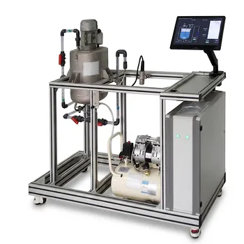
What Is The Significance Of Conducting Rtd Tracer Experiments? Improve Pilot-Plant Flow Understanding

Conducting Residence Time Distribution (RTD) tracer experiments is significant because it reveals how fluid actually flows through a pilot plant, rather than assuming ideal reactor behavior. By injecting an inert tracer as a pulse or step and measuring its outlet concentration over time, students and engineers obtain C-curves, E-curves, and F-curves. These data quantify mean residence time, mixing behavior, and deviations such as channeling, short-circuiting, dead zones, and backmixing.

RTD experiments bridge the gap between ideal reactor theory and real equipment performance. They show how hydraulic non-idealities influence conversion, selectivity, yield, and the validity of reactor models used for design and scale-up.

Why RTD Experiments Matter

They reveal real flow behavior

Ideal plug-flow and continuously stirred-tank reactor models provide useful benchmarks, but physical equipment rarely behaves perfectly. An RTD experiment shows how long different fluid elements actually remain inside the reactor.

A broad or irregular tracer response may indicate significant variation in fluid residence times. Early tracer breakthrough can suggest bypassing or short-circuiting, while a prolonged tail can indicate stagnant regions or dead volume.

They quantify residence time and mixing

The measured concentration response can be converted into the exit age distribution, E(t), and the cumulative distribution, F(t). These functions provide a quantitative description of how fluid elements move through the system.

The experimental mean residence time is calculated from the tracer response:

[ \bar{t}=\frac{\int_0^\infty tC(t),dt}{\int_0^\infty C(t),dt} ]

Students can compare this value with the hydraulic estimate:

[ \bar{t}_{\text{theoretical}}=\frac{V}{Q} ]

where (V) is the working volume and (Q) is the volumetric flow rate. The comparison helps identify whether the effective hydraulic volume and flow behavior match expectations.

They connect flow behavior to reactor performance

Residence time affects the opportunity for chemical reaction. If some fluid bypasses the reactor, it may leave before sufficient conversion occurs; if other fluid remains trapped, it may experience excessive residence time or degrade.

RTD data therefore help explain why measured conversion or yield may differ from predictions based on ideal PFR or CSTR equations. This makes the relationship between hydrodynamics, kinetics, and reactor performance directly observable.

What Students Learn From Pilot-Plant RTD Testing

They apply reaction engineering theory to equipment

A pilot plant turns abstract concepts such as ideal mixing, plug flow, and residence-time distributions into measurable operating behavior. Students work with real flow rates, detector signals, sampling intervals, and experimental uncertainty.

This experience reinforces that reactor models are approximations whose usefulness depends on how well they represent the equipment.

They interpret C, E, and F curves

The raw outlet concentration response is commonly represented as a C-curve. Normalizing this response produces the E-curve, which represents the residence-time density function, while integrating the E-curve produces the F-curve, the cumulative fraction of fluid that has exited by time (t).

Comparing these curves helps students visualize early breakthrough, broad distributions, long tails, and other signatures of non-ideal flow.

They estimate statistical flow parameters

The mean residence time provides a central measure of fluid age. The variance, commonly written as (\sigma^2), indicates how widely residence times are spread around the mean.

A small variance is generally associated with behavior closer to plug flow, while a larger variance indicates greater mixing or dispersion. These interpretations must be made alongside the reactor configuration and operating conditions.

They fit and evaluate non-ideal flow models

Experimental RTD data can be compared with models such as the tanks-in-series model or the axial-dispersion model. For example, a single ideal CSTR produces a broad distribution, whereas multiple stirred tanks in series produce a narrower distribution as the number of stages increases.

This exercise teaches students how model parameters represent physical behavior and how empirical data can be used to select or validate a model.

Why Pilot-Scale Equipment Is Especially Valuable

It exposes equipment-specific effects

Small theoretical examples cannot fully demonstrate the effects of inlet design, outlet location, packing, internal geometry, or imperfect mixing. Pilot-scale CSTRs, packed beds, tubular reactors, and reactor cascades make these effects measurable.

The resulting data are more representative of the hydraulic issues encountered in industrial equipment than purely mathematical exercises.

It develops experimental engineering skills

RTD testing requires students to plan tracer injections, establish sampling or sensor intervals, monitor flow stability, and process time-dependent data. They also learn to distinguish genuine flow behavior from measurement noise and experimental error.

These skills are relevant to commissioning, troubleshooting, process optimization, and scale-up.

It supports model validation and scale-up

A pilot plant provides an intermediate setting in which theoretical predictions can be tested before applying them to larger systems. Measured RTD curves can reveal whether a model captures the dominant flow behavior under particular operating conditions.

This is important because geometric scale-up does not automatically preserve mixing, dispersion, or residence-time characteristics.

Designing a Reliable Tracer Experiment

Choose a chemically suitable tracer

An effective tracer should be non-reactive, fully soluble in the process fluid, and easy to detect accurately. It should also have density and viscosity close to those of the carrier fluid so that it does not alter the flow.

The tracer should not adsorb onto vessel walls, packing, or sensors. Otherwise, the measured response may reflect tracer retention rather than the actual fluid residence-time distribution.

Select pulse or step input appropriately

A pulse input introduces a short, concentrated tracer signal and produces a transient outlet response. It is useful for calculating the E-curve and its statistical moments.

A step input changes the tracer concentration from one steady value to another and is naturally analyzed through the F-curve. Both methods can characterize the system when the input and response are measured accurately.

Collect sufficient response data

The sampling period must be short enough to capture the rising and falling portions of the tracer response. Measurements should continue long enough to account for the response tail, particularly when dead zones or stagnant regions may be present.

Poor temporal resolution or prematurely stopping data collection can distort the calculated mean and variance.

Understanding the Trade-offs

Ideal models are useful but incomplete

Ideal PFR and CSTR models provide clear reference cases, but they cannot describe every feature of real flow. Treating them as exact representations may lead to incorrect predictions of conversion and reactor capacity.

RTD models improve the description of flow, but they still simplify complex three-dimensional hydrodynamics.

RTD alone does not determine reaction performance

An RTD describes fluid movement, not the complete reaction system. Accurate prediction of conversion also requires appropriate reaction kinetics, temperature information, concentration data, and assumptions about mixing at the molecular scale.

Two reactors can have similar RTDs but different reaction outcomes if their local mixing or heat-transfer behavior differs.

Experimental errors can resemble flow non-idealities

Tracer adsorption, incomplete dissolution, detector lag, unstable flow, sampling errors, and poor tracer injection can all create misleading response curves. A long tail, for example, may result from tracer interaction with the equipment rather than a genuine stagnant zone.

Reliable interpretation therefore depends on tracer selection, instrument calibration, flow control, and material-balance checks.

Pilot results require engineering judgment

A pilot-scale RTD is valuable evidence, but it does not guarantee identical behavior at industrial scale. Changes in Reynolds number, geometry, packing, flow distribution, and operating conditions can alter the observed distribution.

The pilot result should be used to test assumptions and improve models, not applied to a larger system without considering scale-dependent effects.

Making the Right Choice for Your Goal

RTD experiments are most valuable when the test is tied to a specific learning, diagnostic, or design objective.

If your primary focus is teaching reactor theory: Use pulse and step experiments to compare ideal PFR and CSTR behavior with measured C, E, and F curves.
If your primary focus is diagnosing equipment performance: Examine early breakthrough, broad distributions, and long tails for evidence of channeling, short-circuiting, dispersion, or dead zones.
If your primary focus is predicting conversion: Combine the measured RTD with appropriate reaction kinetics and a justified non-ideal reactor model.
If your primary focus is model validation or scale-up: Compare experimental mean residence time and variance with predictions from tanks-in-series or axial-dispersion models under controlled operating conditions.
If your primary focus is obtaining reliable data: Select a non-reactive, soluble, detectable, flow-matched, non-adsorbing tracer and verify the measurement system before interpreting the curve.

An RTD tracer experiment gives students and engineers the evidence needed to understand, model, and improve how real reactors perform.

Summary Table:

Key Aspect	What RTD Experiments Reveal
Flow behavior	Channeling, short-circuiting, dead zones, backmixing, and dispersion
Core data	C-curves, E-curves, F-curves, mean residence time, and variance
Reactor performance	How residence-time variation affects conversion, yield, and selectivity
Student learning	Practical application of reactor theory, data analysis, and uncertainty evaluation
Model validation	Comparison with PFR, CSTR, tanks-in-series, and axial-dispersion models
Experiment quality	Effects of tracer selection, sampling frequency, detector response, and flow stability
Scale-up value	Evidence for evaluating hydraulic assumptions before industrial application

Want to give students and engineers hands-on experience with real reactor behavior? Contact LABPARK to discuss Educational and Vocational Unit Operations Pilot Plants for chemical engineering, bioprocess and biotech, and environmental and water treatment applications. Our pilot plants help universities, research institutes, and enterprises evaluate residence-time distributions, mixing, reactor performance, and scale-up assumptions using practical, measurable experiments.