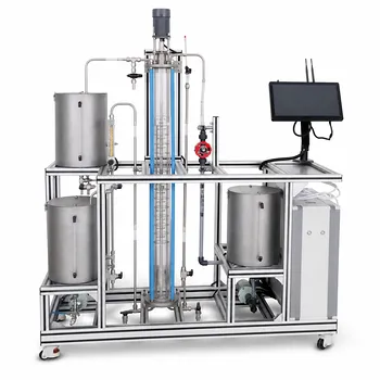
What Essential Structural Elements Must Be Defined? Build Reliable Dynamic Pilot-Plant Optimization Models

The essential structure of a dynamic optimization model is an objective function, decision variables, and constraints. The objective function states what the pilot plant should optimize, such as minimizing operating cost or batch time, or maximizing purity, yield, or profit. Decision variables identify the controllable inputs, while equality and inequality constraints ensure that proposed operating policies obey the process physics, product specifications, equipment limits, and safety requirements.

A feasible operating policy satisfies the process model equations and all operating bounds; an optimal policy is the feasible policy that best achieves the chosen economic or operational objective.

Define What the Optimization Must Achieve

Objective Function

The objective function converts the pilot plant’s goal into a mathematical performance measure.

Typical objectives include:

Minimizing batch cycle time
Minimizing energy consumption or operating cost
Maximizing product purity, recovery, yield, or quantity
Maximizing overall profit

For a batch distillation column, the objective might minimize processing time while meeting distillate purity and recovery requirements. For a reactor, it might maximize product yield while limiting residence time, energy use, or raw-material consumption.

Single and Multiple Objectives

Some pilot plants have competing goals. Increasing reflux may improve distillate purity but increase energy consumption and extend the batch operation.

These cases can be handled with a weighted objective, a constrained secondary objective, or a multiobjective optimization formulation. The chosen method should reflect how the process will actually be evaluated.

Identify the Variables the Model Can Change

Decision Variables

Decision variables are the controllable quantities selected by the optimizer. They may be constant settings, time-varying trajectories, or discrete operating choices.

Examples include:

Reflux ratio or reflux-rate profile
Reboiler heat duty or vapor boilup rate
Reactor temperature profile
Feed rate and feed timing
Batch termination time
Cooling or heating rates
Operating mode or control-policy parameters

For dynamic systems, the variables are often functions of time. Optimizing a reflux ratio profile, for example, gives the model the ability to change reflux as the batch composition and inventory evolve.

State Variables

The model must also represent state variables, which describe the evolving condition of the process.

In a distillation column, states may include tray compositions, liquid holdups, temperatures, and vessel inventories. In a reactor, they may include species concentrations, temperature, pressure, and accumulated product.

State variables are generally determined by the dynamic model rather than chosen freely. They connect operating decisions to the process trajectory and final performance.

Parameters and Initial Conditions

Model parameters describe fixed or estimated characteristics, such as equilibrium data, reaction kinetics, equipment dimensions, heat-transfer coefficients, and feed composition.

Initial conditions are equally important in dynamic optimization. Initial vessel inventories, temperatures, compositions, and reactor conditions determine the starting point from which the operating trajectory develops.

Enforce the Process Physics

Equality Constraints

Equality constraints are the mathematical equations that the process must satisfy exactly, subject to numerical tolerances during computation.

They typically include:

Component and total mass balances
Energy balances
Phase-equilibrium relationships
Reaction-rate expressions
Equipment and holdup dynamics
Material-property relationships
Initial and terminal conditions

For a distillation column, these equations describe vapor-liquid contact, component transfer between stages, condenser and reboiler behavior, and changes in vessel inventory. For a reactor, they describe species consumption and formation, heat generation or removal, and changes in temperature or concentration.

Dynamic Model Equations

A dynamic optimization model commonly has the form:

[ \frac{dx}{dt}=f(x,u,p,t) ]

where (x) represents process states, (u) represents manipulated variables, (p) represents model parameters, and (t) is time.

The equations determine whether a proposed control trajectory is physically possible. An optimizer cannot legitimately improve profit or reduce cycle time by selecting inputs that violate these balances.

Boundary and Specification Equations

Some requirements are naturally expressed as equalities. Examples include a specified final batch volume, a prescribed terminal inventory, or a required production quantity.

Product purity may also be represented as an equality when the process is required to reach an exact target, although inequality constraints are usually more practical when a minimum acceptable specification is sufficient.

Keep Operation Within Acceptable Limits

Inequality Constraints

Inequality constraints define allowable operating regions rather than exact process relationships.

They can impose lower and upper bounds on:

Temperature and pressure
Reflux and reboil ratios
Heat duty and flow rates
Liquid levels and vessel inventories
Reactor concentrations
Product impurity levels
Batch duration
Equipment capacity

For example, a batch distillation model may require minimum distillate purity, maximum reboiler temperature, minimum reboiler liquid level, and bounded reflux and reboil ratios.

Safety and Equipment Constraints

Safety constraints prevent the optimizer from selecting mathematically attractive but hazardous conditions. They may limit temperature, pressure, reaction severity, heating rate, or inventory.

Equipment constraints ensure that calculated operating policies remain executable on the pilot plant. A solution requiring a heat duty, flow rate, or actuator movement beyond the available hardware is not practically feasible.

Product and Process Requirements

Product specifications should be represented explicitly. A minimum purity requirement can be written as:

[ x_{\text{product}}(t_f) \geq x_{\text{required}} ]

where (t_f) is the final or collection time.

Other requirements may include minimum recovery, maximum impurity concentration, target yield, or a permitted purity tolerance. These constraints connect the optimization model to downstream process needs and customer standards.

Represent Feasibility Over the Entire Operation

Path Constraints

Dynamic constraints may need to hold at every time point, not only at the beginning or end of the batch.

A maximum reactor temperature, for example, must not be exceeded during a transient excursion even if the final temperature is acceptable. Similarly, a reboiler liquid level must remain above its dry-out limit throughout the operation.

Initial and Terminal Conditions

Initial conditions define the state of the pilot plant at the start of optimization. Terminal conditions define what must be true when the operation ends.

Examples include:

Initial feed composition and inventory
Initial reactor temperature
Final product purity
Final product quantity
Minimum remaining reboiler inventory
Required batch termination condition

These conditions are part of the model’s structural definition, not optional implementation details.

Feasible Operating Policies

A set of decision variables and resulting state trajectories is feasible when it satisfies:

The equality-based process model
All initial and terminal conditions
Every applicable inequality constraint over the operating horizon

The optimizer searches within this feasible region for the policy that gives the best objective value.

Connect the Model to Pilot-Plant Control

Manipulated Variables and Measurements

The optimization variables should correspond to quantities the pilot plant can actually manipulate. A calculated temperature trajectory is not useful if the equipment has no reliable actuator or control loop capable of following it.

The model should also reflect available measurements, such as composition, level, temperature, pressure, and flow. This is particularly important when an optimized trajectory will be implemented through a control system.

Distillation Control Structure

For a binary distillation pilot plant, control-loop pairings should account for dynamic response times and loop interactions.

Direct material-balance pairings commonly associate distillate flow with distillate composition, reflux with overhead accumulator level, and reboiler steam flow with column bottoms level. Pairings that regulate a level using a flow at the opposite end of the column can introduce substantial delay and poor disturbance rejection.

Robustness to Disturbances

A nominally optimal trajectory may perform poorly when feed composition, heat-transfer behavior, condenser subcooling, or kinetic parameters vary.

For pilot-plant use, the formulation should evaluate relevant parameter variations or disturbances where reliability matters. The preferred solution may be the one with slightly lower nominal performance but better average profitability and fewer violations under realistic operating uncertainty.

Understanding the Trade-offs

Economic Performance Versus Energy Use

Higher reflux or reboiler duty can improve separation and reduce the time needed to reach a purity target, but it generally increases energy demand.

The objective function must make this trade-off explicit. Otherwise, the optimizer may drive an operating variable toward an extreme simply because its cost is absent or understated.

Hardware Design Versus Operating Flexibility

Column stage count, diameter, reboiler area, condenser area, and still capacity affect the achievable operating region.

A column with more equilibrium stages may reach a target purity at a lower reflux ratio, while a column with fewer stages may require higher reflux and longer operation. Equipment parameters should therefore be treated as fixed model parameters or, when design is also being optimized, as additional decision variables with capital-cost constraints.

Nominal Optimality Versus Practical Robustness

The mathematically best trajectory under one set of parameters may be sensitive to model error or disturbances.

An optimization model intended for physical execution should balance objective performance with constraint margins, actuator limitations, measurement uncertainty, and the ability of the control system to track the solution.

Common Pitfalls to Avoid

Omitting Decision Variables

Defining an objective and constraints without stating which inputs the optimizer may change leaves the optimization problem incomplete.

The variables must be clearly distinguished from fixed parameters, measured disturbances, and process states.

Using Only Endpoint Constraints

Checking purity or temperature only at the final time can allow unsafe or unacceptable intermediate behavior.

Safety limits, inventory bounds, and temperature restrictions should be imposed as path constraints whenever they must hold throughout the operation.

Optimizing an Unrealistic Model

A model that omits balances, phase equilibrium, kinetics, or equipment dynamics can produce an apparently excellent but physically invalid result.

The process equations must be detailed enough to represent the behavior relevant to the optimization goal.

Ignoring Implementability

A control trajectory may satisfy the mathematical model but be impossible for the pilot plant to follow because of actuator saturation, rate limits, sampling delays, or inadequate measurements.

These practical limitations should be included as constraints or handled through a compatible control architecture.

How to Apply This to Your Project

A well-formed dynamic optimization model should define the objective, decision variables, state representation, process equations, operating limits, and initial and terminal conditions before an algorithm is selected.

If your primary focus is economic performance: Define profit or cost explicitly, including energy and batch-time effects, while retaining product, safety, and equipment constraints.
If your primary focus is product quality: Use purity, recovery, yield, and impurity limits as explicit constraints or objective terms rather than relying on indirect operating targets.
If your primary focus is safe pilot-plant execution: Include time-dependent temperature, pressure, level, inventory, actuator, and rate limits across the entire operating trajectory.
If your primary focus is dynamic control: Select decision variables that correspond to available actuators and account for response times, loop interactions, disturbances, and tracking limitations.
If your primary focus is equipment design: Include stage count, diameter, heat-transfer area, capacity, or other hardware choices as design variables and balance their cost against operating performance.

A credible optimization model links a measurable goal to controllable inputs through physically valid equations and enforceable operating limits.

Summary Table:

Model element	Purpose	Pilot-plant examples
Objective function	Defines what the optimization should improve	Minimize cost, energy use, or batch time; maximize purity, yield, recovery, or profit
Decision variables	Identifies controllable inputs selected by the optimizer	Reflux rate, heat duty, feed rate, reactor temperature, cooling rate, batch termination time
State variables	Represents how the process changes over time	Tray compositions, holdups, temperatures, inventories, concentrations, pressure
Parameters and initial conditions	Defines fixed process characteristics and the starting state	Kinetics, equilibrium data, equipment dimensions, feed composition, initial temperature and inventory
Equality constraints	Enforces process physics and required conditions	Mass and energy balances, phase equilibrium, reaction kinetics, initial and terminal conditions
Inequality constraints	Keeps operation within acceptable limits	Temperature, pressure, level, inventory, flow, purity, recovery, capacity, and batch-time limits
Path constraints	Ensures limits are satisfied throughout the operation	Maximum reactor temperature, minimum reboiler level, actuator and heating-rate limits
Control and measurement requirements	Connects the optimization to executable plant operation	Available actuators, sensor data, response times, loop interactions, rate limits, and sampling delays
Robustness considerations	Protects performance against uncertainty and disturbances	Feed variation, heat-transfer changes, condenser behavior, kinetic uncertainty, and model error

Planning a dynamic unit operations pilot plant? Contact LABPARK to discuss an optimization-ready system designed for your application. LABPARK provides Educational and Vocational Unit Operations Pilot Plants for chemical engineering, bioprocess and biotechnology, and environmental and water treatment. Our solutions help universities, research institutes, and enterprises connect process models with real equipment through controllable operating variables, measurable states, realistic process constraints, and practical safety limits. Work with LABPARK to evaluate distillation columns, chemical reactors, and other pilot-scale systems that support teaching, research, process development, operator training, and reliable scale-up.