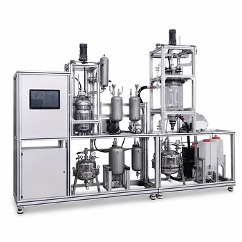
How Can Molecular Screening Charge Densities Guide Solvent Selection? Optimize Lle Pilot Plant Workflows.

Molecular-level polarity predictions are transforming how engineers select solvents before a single drop flows in a pilot plant. In liquid-liquid extraction, the screening charge density—captured by a molecule’s (\sigma)-profile—acts as a local descriptor of surface polarity. By analyzing these profiles, you can computationally pre-screen solvents for their ability to interact with a target solute, directly predicting electrostatic misfit and hydrogen-bonding energies. In an educational or R&D pilot plant, this means students and researchers arrive at the extraction column with a shortlist of rationally chosen candidates, ready to validate molecular-level predictions against macroscopic separation efficiency.

The core insight: A (\sigma)-profile translates a molecule’s intricate surface charge distribution into a quantitative map of polarity and hydrogen-bonding potential. This map allows you to predict, through thermodynamic models, how strongly a solvent will attract a solute—turning solvent selection from a heuristic “like dissolves like” exercise into a rigorous, energy-based screening process that still demands final physical confirmation in a pilot plant.

Understanding the Molecular Fingerprint: What a (\sigma)-Profile Actually Reveals

A (\sigma)-profile plots the amount of molecular surface area that carries a given screening charge density (\sigma). This single function captures the essential character of a molecule as seen by an approaching partner.

Polarity Beyond a Single Number

Traditional parameters like dielectric constant or log (P) reduce polarity to one value. By contrast, a (\sigma)-profile shows the complete distribution of positive, negative, and neutral surface patches. A broad, multi-peaked profile signals a complex, charge-separated surface (strong local polarity), while a narrow peak around zero signals a non-polar, smoothly distributed charge.

Hydrogen-Bonding Fingerprints

Crucially, a (\sigma)-profile identifies hydrogen-bond donor and acceptor tendencies. Strongly negative screening charge densities (e.g., from lone-pair electrons on oxygen or nitrogen) indicate hydrogen-bond acceptor capacity, while strongly positive regions (e.g., from acidic hydrogens) mark donor ability. These regions appear as distinct peaks far from the zero-charge baseline, giving you a direct visual of a solvent’s hydrogen-bonding arsenal.

From Charge Densities to Separation Predictions

Knowing a solvent’s (\sigma)-profile is only half the story. The real value comes when you pair it with the (\sigma)-profiles of the solute and carrier liquid to calculate the energy of interaction.

Quantifying the Electrostatic Misfit

When two molecules approach in solution, mismatches in their local surface charge densities create an electrostatic misfit penalty. In COSMO-based thermodynamic models, this misfit energy is computed by integrating over the contact area and the squared difference of the screening charge densities. A solvent whose (\sigma)-profile closely complements the solute’s charge distribution effectively “fits” like a jigsaw piece, reducing the energetic cost and boosting solubility.

Predicting Distribution Coefficients and Selectivity

The overall interaction energy—sum of misfit, hydrogen-bonding, and van der Waals contributions—fed into statistical thermodynamics directly yields activity coefficients. From there, you obtain the distribution coefficient (K_{iD}) for your solute between extract and raffinate phases, and relative selectivity (\beta). A solvent that generates a significantly lower activity coefficient for the solute (compared to the carrier) will exhibit high capacity and selectivity. This computational pipeline means you can rank hundreds of candidate solvents by predicted (\beta) before committing to any pilot-plant experiment.

Integrating Molecular Screening into an Educational Pilot Plant Workflow

The primary reference highlights that in vocational and educational settings, the (\sigma)-profile approach lets students computationally screen solvents beforehand. This directly connects molecular theory to the tangible operation of a pulsed, packed, or rotating-disc column.

Step 1: In Silico Ranking

Students first run COSMO-RS (or equivalent) calculations using the (\sigma)-profiles of the solute, feed solvent, and a library of potential extractants. They filter out solvents with poor predicted selectivity, unfavorable distribution, or known hazardous properties. The output is a short, technically justified list.

Step 2: Pilot-Plant Validation

Armed with the predictions, they charge the extraction column and measure the actual mass transfer performance: solute concentration in each phase, flooding limits, and settler operation. They observe whether the solvent ranked highest in silico truly delivers the swift, sharp separation predicted. This closes the loop between molecular descriptions (hydrogen-bond donor/acceptor peaks on a graph) and macroscopic phenomena like emulsion formation or phase separation speed.

Understanding the Trade-offs and Limitations

Molecular screening via (\sigma)-profiles is powerful, but relying on it blindly can lead you astray. Several practical realities must temper the computational enthusiasm.

Physical Properties Still Rule Hydrodynamics

A solvent with an ideal (\sigma)-profile could still fail in the pilot plant due to high viscosity, a density too close to the aqueous phase, or unfavorable interfacial tension. These properties dictate coalescence rates, column throughput, and whether you face flooding or entrainment. The pilot plant remains essential to observe these hydrodynamic limits that current charge-density models cannot capture directly.

Accuracy Depends on Quantum Chemistry Quality

The (\sigma)-profiles themselves are derived from density functional theory calculations performed on single molecules in a virtual conductor. Approximations in the level of theory, the cavity construction, and the statistical thermodynamics can introduce errors, particularly for complex associating mixtures. Predictions give you a strong lead, but they are not a substitute for measuring at least a few distribution coefficients.

Safety and Stability are Non-Negotiable

A computationally perfect solvent might be toxic, corrosive, or peroxide-forming. The supplementary references remind us that low-polarity ethers offer excellent extraction ability but come with extreme fire risks. The screening workflow must therefore overlay a practical safety filter—rejecting candidates that fail basic chemical safety criteria—before they ever reach the pilot-plant floor.

Making the Right Choice for Your Goal

When you stand at the interface between molecular simulation and the pilot plant, tailor your use of (\sigma)-profiles to what truly matters in your separation.

If your primary focus is maximizing selectivity: Prioritize solvents whose (\sigma)-profiles show large, complementary mismatch in hydrogen-bonding donor/acceptor regions relative to the solute, while minimizing attraction to the carrier. Use the predicted (\beta) ranking to shortlist only the top three candidates for physical testing.
If your primary focus is rapid, trouble-free pilot-plant demonstration: Combine the (\sigma)-profile screening with a hard filter on physical properties—density difference >100 kg/m³, viscosity <2 cP, and high interfacial tension. The in silico solubility advantage must not be nullified by a column that floods early.
If your primary focus is educational depth: Have students first classify solvents using the Ewell hydrogen-bonding groups, then compute (\sigma)-profiles to see why the rules work (and where they break down). Challenge them to explain why a molecule from the same Ewell class can behave differently because of its unique charge distribution pattern.

Using the screening charge density as your compass turns solvent selection into a predictable, teachable science—but the pilot plant remains the ultimate arbiter where the calculated misfit energy meets the reality of a separating funnel or a pulsing column.

Summary Table:

Selection Method	Key Parameters	Main Advantages	Pilot Plant Value
Traditional Heuristics	Dielectric constant, Log P	Simple & quick	High risk of trial-and-error
Sigma-Profiles (COSMO)	Local charge density, H-bond donor/acceptor	High accuracy, in silico pre-screening	Minimizes physical runs, optimizes design

Optimize Your LLE Unit Operations with LABPARK

Bridging molecular theory and physical pilot-scale validation is key to training the next generation of engineers and accelerating R&D. LABPARK provides premium Educational and Vocational Unit Operations Pilot Plants in chemical engineering, bioprocess & biotech, and environmental & water treatment. Designed specifically for universities, research institutes, and enterprises, our pilot plants enable students and researchers to seamlessly validate in silico solvent screening models like $\sigma$-profiles on physical, high-performance extraction columns.

Ready to elevate your engineering lab? Contact our technical experts today to find the perfect pilot plant system for your curriculum or research needs!