For creeping flow past a spherical particle, total hydrodynamic drag is given by Stokes’ law, (F_D = 6\pi \mu R U), where (\mu) is fluid viscosity, (R) is particle radius, and (U) is the relative velocity between the particle and fluid. The total force is obtained by integrating the fluid traction over the entire spherical surface. Pressure forces contribute one-third, (F_{D,p}=2\pi\mu R U), while viscous shear forces contribute two-thirds, (F_{D,\tau}=4\pi\mu R U).

In creeping flow, the sphere’s drag is linear in viscosity, particle size, and relative velocity. Although inertia is negligible, the surrounding pressure field still contributes one-third of the drag; surface shear contributes the remaining two-thirds.

Establishing the Creeping-Flow Regime

The Relevant Reynolds Number

Creeping flow applies when the particle Reynolds number is much less than one:

[ Re_p=\frac{\rho U d}{\mu}\ll 1 ]

where (\rho) is fluid density and (d=2R) is the particle diameter.

At such low Reynolds numbers, inertial effects are negligible compared with viscous effects. The flow is governed primarily by the balance between pressure gradients and viscous stresses.

The Meaning of Relative Velocity

The velocity (U) in Stokes’ law is the relative velocity between the particle and the surrounding fluid. For a stationary particle in a moving fluid, (U) is the local fluid velocity relative to the particle.

For a settling particle, (U) is the particle’s velocity relative to the fluid, often evaluated at terminal velocity when the net force is zero.

Calculating Total Hydrodynamic Drag

Stokes’ Law

The total drag magnitude on a sphere is

[ F_D=6\pi\mu R U ]

Using diameter instead of radius gives the equivalent form

[ F_D=3\pi\mu d U ]

The drag acts opposite to the particle’s relative motion through the fluid.

Surface-Force Integration

The force on the particle comes from the fluid traction acting over its surface. That traction has two components:

[ \text{surface traction}= \text{normal pressure traction} + \text{tangential viscous traction} ]

Integrating both components over the spherical surface yields

[ F_D=F_{D,p}+F_{D,\tau} ]

For a sphere in creeping flow,

[ F_{D,p}=2\pi\mu R U ]

and

[ F_{D,\tau}=4\pi\mu R U ]

Therefore,

[ F_D

2\pi\mu R U+4\pi\mu R U

6\pi\mu R U ]

Relative Contributions of Pressure and Shear

Pressure Contribution

The pressure distribution around the sphere produces

[ F_{D,p}=2\pi\mu R U ]

Relative to the total drag,

[ \frac{F_{D,p}}{F_D}

\frac{2\pi\mu R U}{6\pi\mu R U}

\frac{1}{3} ]

Thus, pressure accounts for approximately 33.3% of the total drag.

This pressure field is not an inertial form-drag effect in the usual high-Reynolds-number sense. Even though inertia is negligible, viscous flow around the sphere requires a pressure gradient, and that pressure distribution has a net force component in the direction opposing motion.

Shear-Stress Contribution

The tangential viscous stresses at the particle surface produce

[ F_{D,\tau}=4\pi\mu R U ]

Their fraction of the total drag is

[ \frac{F_{D,\tau}}{F_D}

\frac{4\pi\mu R U}{6\pi\mu R U}

\frac{2}{3} ]

Therefore, viscous shear accounts for approximately 66.7% of the total drag.

This larger contribution reflects the no-slip condition at the particle surface. Fluid velocity changes rapidly from the particle’s surface velocity to the surrounding flow velocity, creating velocity gradients and tangential wall shear stress.

The One-Third to Two-Thirds Split

The force breakdown can be summarized as

[ F_D

\underbrace{2\pi\mu R U}{\text{pressure: }1/3} + \underbrace{4\pi\mu R U}{\text{shear: }2/3} ]

The ratio of pressure drag to shear drag is therefore

[ F_{D,p}:F_{D,\tau}=1:2 ]

This distinction is useful in teaching equipment because pressure sensors and force measurements may reflect different parts of the same hydrodynamic interaction.

Relating the Result to Unit Operations Equipment

Sedimentation and Clarification

In settling experiments, Stokes’ law is used to relate particle size, fluid viscosity, and settling velocity. At terminal settling velocity, the drag balances the effective weight of the particle:

[ F_D=F_g-F_b ]

where (F_g) is particle weight and (F_b) is buoyancy.

The drag calculation helps students analyze sedimentation efficiency, residence time, and the performance of clarifiers or separation columns.

Differential-Pressure Measurements

Pilot equipment may measure pressure differences across flow channels, packed sections, or separation devices. These measurements represent pressure forces associated with fluid momentum and viscous resistance across the equipment, not necessarily the pressure component of the drag on one isolated sphere.

Consequently, a measured pressure drop should not automatically be interpreted as the one-third pressure contribution in Stokes’ law. The measurement geometry and the control volume determine which forces are being recorded.

Shear-Stress Measurements

Wall shear stress is related to the local velocity gradient by

[ \tau_w

-\mu \left(\frac{\partial u_x}{\partial y}\right)_{y=0} ]

This relation illustrates the same physical principle responsible for the sphere’s shear contribution: viscous force arises from velocity gradients at a surface.

Flat-plate correlations, such as laminar boundary-layer friction relations, are useful for channel and wall-flow experiments. They should not be substituted directly for the spherical-particle result, because the geometry and velocity field are different.

Understanding the Trade-offs

Stokes’ Law Has a Limited Reynolds-Number Range

The (6\pi\mu R U) relationship is valid when (Re_p\ll 1). As Reynolds number increases, inertia becomes important and the drag is no longer strictly proportional to velocity.

At higher Reynolds numbers, wake formation, flow separation, and inertial pressure drag can substantially change both the total drag and the pressure-to-shear distribution.

Particle Shape Matters

The one-third pressure and two-thirds shear split applies to an ideal, smooth, rigid sphere in an otherwise unbounded Newtonian fluid. Irregular particles, fibers, droplets, and biological particles can have different drag coefficients and stress distributions.

Near a wall, inside a narrow channel, or among neighboring particles, the surrounding boundaries modify the flow and increase or otherwise alter the drag.

Fluid Properties Must Be Applied Consistently

The viscosity (\mu) must be evaluated under the relevant temperature and composition conditions. For non-Newtonian fluids, a single constant-viscosity Stokes-law calculation may not accurately represent the particle-scale stress field.

The fluid must also be sufficiently continuous at the particle scale for continuum mechanics to apply. Very small particles in rarefied or microscale regimes may require corrections beyond the classical result.

Pressure and Shear Are Not Independent Flow Systems

Pressure and shear are separated mathematically to identify their contributions to the integrated force. They are physically coupled parts of the same flow solution around the sphere.

The pressure distribution and surface velocity gradients must therefore be derived from the complete creeping-flow field rather than estimated independently from unrelated equipment correlations.

Applying This to Your Project

Use the following approach when analyzing a spherical-particle experiment:

If your primary focus is total particle drag: Calculate (F_D=6\pi\mu R U) using the fluid viscosity, particle radius, and particle-fluid relative velocity.
If your primary focus is pressure-force contribution: Use (F_{D,p}=2\pi\mu R U=F_D/3), recognizing that this is a viscous-flow pressure contribution rather than high-Reynolds-number inertial form drag.
If your primary focus is surface-friction contribution: Use (F_{D,\tau}=4\pi\mu R U=2F_D/3), which represents the integrated tangential shear stress over the particle surface.
If your primary focus is validating a pilot-plant experiment: Confirm (Re_p\ll1), distinguish particle-scale drag from equipment-scale pressure drop, and account for walls, neighboring particles, and non-Newtonian behavior.

For an ideal sphere in creeping flow, the governing result is clear: one-third of the hydrodynamic drag comes from pressure forces and two-thirds comes from viscous shear stresses.

Summary Table:

Key aspect	Result
Flow regime	Creeping flow, where particle Reynolds number (Re_p \ll 1)
Total drag	(F_D = 6\pi\mu R U)
Pressure contribution	(F_{D,p} = 2\pi\mu R U), or 1/3 (33.3%)
Shear contribution	(F_{D,\tau} = 4\pi\mu R U), or 2/3 (66.7%)
Contribution ratio	Pressure : shear = 1 : 2
Main applications	Sedimentation, clarification, particle settling, and hydrodynamic teaching experiments

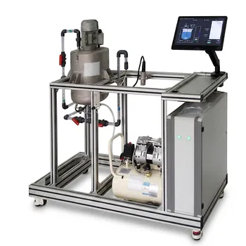
Need reliable equipment for particle settling, drag-force analysis, or fluid mechanics instruction? Contact LABPARK to discuss your requirements. LABPARK provides Educational and Vocational Unit Operations Pilot Plants for chemical engineering, bioprocess and biotech, and environmental and water treatment applications. Our systems help universities, research institutes, and enterprises demonstrate Stokes' law, sedimentation, clarification, pressure effects, and viscous shear through practical, industry-relevant experiments. Work with LABPARK to select a suitable pilot plant, adapt the configuration to your teaching or research objectives, and build hands-on training capability around measurable fluid-process data.