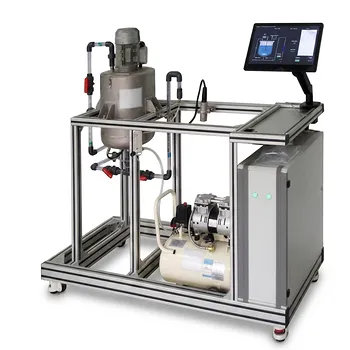
How Is Specific Speed ($N_S$) Used In Pump Unit Ops To Teach Pump Selection & Design?

Pump selection is not guesswork—it’s a data-driven geometry puzzle. In centrifugal pump unit operations equipment, the dimensionless specific speed ($N_s$) serves as a fundamental classifier that links a pump’s duty point (flow and head) to its optimal impeller architecture. Students use $N_s$ to identify whether a pump requires radial, mixed, or axial impellers, to anticipate efficiency limitations that trigger multi-staging, and to confirm these predictions by generating and comparing experimental performance curves in the pilot plant.

Specific speed bridges classroom theory and hands-on learning by collapsing flow, head, and rotational speed into a single, predictable number. This number then unlocks the ideal pump geometry, exposes efficiency boundaries, and gives students a repeatable, objective method for pump selection rather than relying on catalog rules of thumb.

Decoding the Number: What Specific Speed Reveals

The Definition and Its Meaning

The dimensionless specific speed is calculated as $N_s = \frac{N , Q^{1/2}}{(g , h)^{3/4}}$, where $N$ is rotational speed, $Q$ is volumetric flow rate, and $h$ is head.

All variables must be in consistent units, making $N_s$ a pure number that is fundamentally independent of system size. In educational settings, this dimensionlessness teaches students that two geometrically similar pumps will share the same $N_s$, regardless of scale.

Students often encounter a parallel industry convention using US units ($N’_s = N‘Q^{1/2} / h^{3/4}$). The resulting values are numerically different but conceptually identical: both serve to classify impeller types. Recognizing this duality helps students avoid confusion when moving from textbooks to field data sheets.

Impeller Classification by $N_s$

The dimensionless $N_s$ value sorts pumps into three distinct families, each with a characteristic head–flow relationship.

Radial-flow impellers dominate when $N_s$ is low (roughly below 1.0). These pumps excel at producing high head with relatively low flow. Their impellers accelerate fluid outward from the center, making them the standard choice for boiler feed or high-pressure transfer.

Mixed-flow impellers appear in the intermediate range (roughly 1.0 to 2.5). They combine radial and axial components, delivering a balance of moderate head and higher flow. Students encounter these in large-scale water circulation and irrigation duties.

Axial-flow impellers take over at high $N_s$ (above about 2.5). They generate very low head but move enormous volumes, ideal for flood control, cooling water pumping, and recirculation loops. The propeller-like geometry is a direct consequence of the high specific speed.

By calculating $N_s$ at the pump’s best efficiency point (BEP), students learn to predict the impeller shape before ever opening the casing. Many pilot plants then allow disassembly, turning the prediction into a memorable verification.

From Classroom to Curve: Using Pilot Plant Data

Generating Performance Curves

In unit operations labs, students run a centrifugal pump across a range of flow rates while recording head, shaft power, and efficiency. They plot these variables against flow rate to obtain the pump’s characteristic curves.

The Best Efficiency Point (BEP) is then used to compute the pump’s $N_s$. This single calculation anchors the pump in its geometric family and reveals its ideal operating region. Students can then compare their experimental curve shape with textbook characteristic shapes for radial, mixed, or axial pumps, reinforcing the link between $N_s$ and observed performance.

Verifying Design Rules Experimentally

Educational pilot plants let students push beyond classification and directly test selection rules. A powerful example is the single-stage efficiency limit.

When the dimensionless $N_s$ drops below approximately 0.4 (equivalent to the industry benchmark of $N’_s$ < 1,000), a single-stage centrifugal pump struggles to achieve acceptable efficiency. The lab exercise makes this tangible: students calculate $N_s$ for a demanding high-head, low-flow condition, measure the abysmal efficiency, and then observe that a multi-stage pump (or a positive-displacement machine) is required to handle the same duty efficiently.

Students can also manipulate system resistance to move the operating point, recalculate $N_s$, and directly see how a pump’s inherent geometry forces it to operate poorly outside its natural $N_s$ range. These exercises cement the principle that $N_s$ is not just a classification tag—it is a predictive design gatekeeper.

Understanding the Trade-offs

Efficiency Versus Head Capability

Low-specific-speed pumps deliver high head per stage but pay an efficiency penalty. Their narrow flow passages and high disk friction reduce hydraulic efficiency, and they become increasingly sensitive to internal recirculation. Students learn that chasing a radial pump design for a high-flow, low-head service will result in a needlessly expensive, inefficient machine.

Conversely, high-$N_s$ axial pumps achieve excellent efficiencies for large flows but simply cannot generate high pressure without extreme rotational speeds. Each family has a performance territory, and $N_s$ defines its borders—not as a limitation, but as a design constraint students must respect.

Cavitation and Suction Limits

Specific speed is intimately tied to net positive suction head (NPSH) requirements. For a given inlet condition, pushing a pump to a very high $N_s$ can force operation in a region where cavitation becomes unavoidable.

Many educational loops include transparent suction lines or pressure transducers to demonstrate how an improper $N_s$–NPSH match causes performance collapse. This teaches that pump selection must balance geometric suitability with the hydraulic realities of the suction system.

The Metric Trap: Dimensional vs. Dimensionless

A frequent source of student error is mixing the unit-specific industry formula ($N’_s$) with the dimensionless definition. Using the formula without gravity and with US gallon/feet units yields a number in the hundreds or thousands, while the dimensionless $N_s$ is a small fraction.

Mistaking the two can misclassify a pump and lead to a completely wrong selection. Instructor-led exercises that require students to convert between the two forms—and to defend why the dimensionless version is more universal—build the critical thinking needed to avoid such pitfalls in practice.

Making the Right Choice for Your Learning Goal

How you leverage $N_s$ in the pilot plant depends on which skill you want to sharpen.

If your primary focus is understanding impeller physics: Use $N_s$ to predict the geometry of an unknown pump from its performance data, then physically open the casing to verify. This turns abstraction into tactile learning.
If your primary focus is hands-on pump selection: Experiment with varying system curves and calculate $N_s$ at the new operating points. Observe when the efficiency collapses and when staging becomes necessary, reinforcing the single-stage cutoff rule.
If your primary focus is experimental verification: Map the full performance curve for multiple pumps, compute their BEP-specific speeds, and overlay the results on a textbook $N_s$–efficiency chart. The alignment (or misalignment) builds confidence in the predictive power of theory.

Specific speed transforms the centrifugal pump from a black box into a predictable, classifiable machine—and the unit operations pilot plant is where that transformation becomes unforgettable.

Summary Table:

Impeller Type	$N_s$ Range (Dimensionless)	Head vs. Flow Profile	Typical Application
Radial-flow	Low (< 1.0)	High head, low flow	Boiler feed, high-pressure transfer
Mixed-flow	Intermediate (1.0 - 2.5)	Moderate head & flow	Water circulation, irrigation
Axial-flow	High (> 2.5)	Low head, very high flow	Flood control, cooling water loops

Bring Hands-On Pump Selection to Your Lab

LABPARK provides premium Educational and Vocational Unit Operations Pilot Plants in chemical engineering, bioprocess & biotech, and environmental & water treatment. Designed for universities, research institutes, and enterprises, our pilot plants enable students to master pump selection, generate real performance curves, and apply specific speed ($N_s$) theory in real-world scenarios.

Ready to upgrade your lab's training capabilities? Contact LABPARK today to find the perfect pilot plant solution for your program.