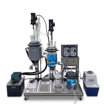
Transport delay is a physical inevitability, not a component failure. It occurs in fluid and thermal pilot plants whenever mass or energy must travel a finite distance at a finite velocity, creating a pure dead time (τ₀) defined by τ₀ = L/v. In a thermal system, this means a sensor placed far downstream from a heat exchanger introduces a lag where the controller acts on old information. The most effective minimization strategies in lab system design are aggressive optimization of sensor placement, radical reduction of pipe lengths and dead volume, and architectural decisions that allocate inevitable delays to slower, outer control loops.
Transport delay (τ₀ = L/v) is a physical lag that starves the controller of real-time feedback, leading to instability. In lab-scale pilot plants, its impact is best minimized through strategic sensor placement, compact fluid path design, and allocating unavoidable delays to slower primary loops in cascade control configurations.
The Physics of Transport Delay: Distance and Velocity
The Fundamental Equation
Transport delay is not a complex chemical phenomenon—it is a purely physical transportation lag. The time it takes for a fluid packet or a thermal front to move from point A to point B is simply the transportation distance (L) divided by the flow velocity (v). This relationship, τ₀ = L/v, is the core of the problem. Because both distance and velocity are design variables, delay becomes an engineering choice from the very first layout sketch.
How It Manifests in Fluid and Thermal Systems
In a fluid flow pilot plant, delay appears when a reagent must travel through a long transfer line before reaching a downstream analyzer or reactor. The measurement system sees the composition or flow rate seconds or minutes after the actual change occurred. In a thermal system, the same principle applies to heat: a temperature sensor installed far downstream of a heat exchanger outlet measures the fluid temperature after it has already moved past the point of control, rendering any feedback loop sluggish and out of sync.
Why Lab-Scale Systems Are Especially Vulnerable
The Disconnect Between Control Action and Measurement
In automated pilot plants, the controller decides on a correction based on the measured error. If dead time is significant, the control action applied now will affect the process only after a delay, but the controller will keep receiving the old, uncorrected value during that interval. This creates a dangerous disconnect: the controller overcompensates because it sees no immediate effect, leading to oscillations or complete instability.
The Critical Ratio: Dead Time vs. Time Constant
The problem is not absolute delay but how large the dead time is relative to the process time constant. A small pilot plant often has faster dynamics (small volumes, quick heat-up times), so a seemingly minor transport delay can dominate the loop’s response. When τ₀ approaches or exceeds the process time constant, standard feedback control can easily become unstable. Identifying this ratio early is crucial to selecting an appropriate control strategy—such as predictive algorithms or cascade structures—rather than applying a one-size-fits-all PID.
Proven Design Strategies to Minimize Delay
Optimize Sensor Location for Instantaneous Feedback
The single most impactful step is to relocate sensors as close as possible to the disturbance source or actuator. The goal is to make the measurement point reflect the process change with minimal transportation lag. In a heat exchanger loop, this means placing the temperature sensor immediately at the exchanger outlet, not after a serpentine sample line. This removes unnecessary L from the τ₀ = L/v equation without altering flow rates.
Shorten Pipe Lengths and Minimize Dead Legs
Every millimeter of unnecessary tubing adds to transportation lag. In lab system design, you should ruthlessly simplify the fluid path: route piping directly, eliminate dead-ended tees, and avoid oversized holding chambers. Dead volume acts as both a transportation delay and a mixing zone that smears concentration profiles, compounding the lag effect. Use narrow-bore tubing only where shear or pressure drop is acceptable, and always prioritize a compact, linear layout.
Leverage System Architecture: Cascade Control Partitioning
When some transport delay is physically unavoidable, design the control architecture to isolate it. A cascade control scheme can place the fast-responding inner (secondary) loop around the actuator and immediate process element, ensuring this loop contains as little dead time as possible. The significant transport delay is then allocated to the outer (primary) loop, where its effect is naturally attenuated. This keeps the inner loop responsive and allows it to suppress local disturbances before they propagate through the system.
Understanding the Trade-offs
The Risk of Non-Representative Measurements
Pushing a sensor too close to an outlet can compromise accuracy. If a temperature sensor is placed immediately after a heat exchanger, it might capture incomplete mixing or localized gradients, giving a reading that does not represent the true bulk fluid temperature. The design choice becomes a balance between speed of response and measurement representativeness, sometimes requiring a short, well-mixed micro-chamber instead of a direct in-pipe probe.
Compactness vs. Operational Accessibility
Short pipe runs and minimal dead legs save transport delay but can create a maintenance nightmare. A tightly packed system may make valve operation, sample collection, or cleaning nearly impossible. In a research pilot plant, where flexibility is key, you must weigh the control benefit of a centimetre-shorter line against the long-term cost of reduced accessibility and modifiability.
The Myth of Zero Delay
No physical system can have zero transport delay. Even with optimal design, there will always be a finite L and v. The realistic goal is to reduce τ₀ to a value significantly smaller than the dominant process time constant, making it a secondary effect rather than the dominant stability limit. Accepting this inevitability early moves the design focus from elimination to mitigation.
Making the Right Choice for Your Pilot Plant Design
Start with a clear definition of your control performance target. Your strategy should map directly onto that target.
- If your primary focus is control responsiveness and tight regulation: Place sensors as close as physically possible to the actuator, even if it requires minor compromises in bulk measurement accuracy. Use a cascade architecture with a near-zero-delay secondary loop.
- If your primary focus is research flexibility and the ability to reconfigure the plant: Design a modular tube-and-fitting system with standardized short-run segments. Accept a small baseline delay but use high-velocity flows to shrink τ₀, and document the dead time for later model-based compensation.
- If your primary focus is accurate thermodynamic or kinetic measurement: Prioritize representative sampling over zero delay. Use a well-mixed, low-volume sample cell near the point of interest and compensate for the known, constant transport delay in the data analysis or using a Smith predictor.
By treating transport delay as a design parameter rather than an unfortunate constant, you can build a pilot plant that responds predictably and enables robust control—turning a fundamental fluid dynamic into a manageable variable.
Summary Table:
| Minimization Strategy | Action | Main Benefit | Key Trade-off |
|---|---|---|---|
| Sensor Placement | Locate sensors close to actuators | Instant feedback, reduced lag | Risks non-representative readings |
| Fluid Path Optimization | Shorten piping, eliminate dead legs | Minimizes dead volume & delay | Reduces maintenance accessibility |
| Cascade Control | Allocate delay to outer loop | Isolates lag, stabilizes inner loop | Requires more complex control logic |
Optimize Your Lab's Control System with LABPARK
Are you looking to eliminate control instabilities and design-stage lag in your process systems? LABPARK provides state-of-the-art Educational and Vocational Unit Operations Pilot Plants in chemical engineering, bioprocess & biotech, and environmental & water treatment.
We assist universities, research institutes, and enterprises in building highly responsive, stable, and customized pilot systems that bridge the gap between theoretical dynamics and robust physical control.
Ready to elevate your pilot plant performance? Contact our engineering experts today!
Related Products
- Thermal Desorption Exhaust Gas and Tail Water Treatment Educational Pilot Plant
- Hot Filtration Educational Unit Operations Pilot Plant Laboratory System
- Dual Mode Heat Transfer Pilot Plant for Unit Operations Training
- Comprehensive Fluid Mechanics Educational Unit Operations Pilot Plant
- Multi Pump Fluid Transport Process Piping Unit Operations Training Pilot Plant
People Also Ask
- How is iron concentration monitored to evaluate corrosion and filtration efficiency in water treatment pilot plants?
- How is P, M, and B alkalinity applied in pilot plants? Prevent Boiler Scaling & Corrosion
- Lime-Soda vs. Cation Exchange Softening: How Do Effluent Characteristics Compare in Pilot Plants?
- How do anodic & cathodic inhibitors protect heat exchangers? Optimize Your Water Treatment Pilot Plant
- What are inline fluorescence sensor risks, and how can they be managed? Key Strategies