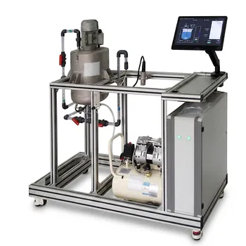
The pseudobinary diffusion approximation reduces a multicomponent transport problem to a familiar single-solute diffusion equation. In a dilute liquid solution dominated by one solvent, such as water, interactions among minor solutes can often be neglected. The solute flux is then modeled with one diffusivity, (D_i), and the species conservation equation becomes a standard diffusion-reaction equation rather than a coupled multicomponent system.

When one solvent overwhelmingly dominates the liquid mixture, each dilute solute can often be treated as diffusing through an effectively stationary solvent. This replaces a multicomponent diffusion matrix with a single Fickian diffusivity for the solute, making pilot-plant concentration profiles and mass-transfer rates much easier to calculate.

Why Multicomponent Diffusion Is Difficult

Every species can influence transport

In a general mixture, the flux of species (i) depends on concentration gradients and diffusional interactions involving several other species. These relationships are commonly represented using generalized Stefan-Maxwell equations or multicomponent diffusion coefficients.

The resulting equations are coupled: changing the concentration of one component can alter the fluxes of others. This creates a larger mathematical and experimental problem than simply applying binary Fick's law.

Pilot-plant experiments need usable models

Educational pilot plants are intended to connect measured operating data with transport theory. A fully multicomponent model may require diffusion matrices, detailed thermodynamic data, and numerical solution methods that obscure the main learning objective.

For dilute systems, the pseudobinary approximation preserves the dominant physical behavior while keeping the governing equations tractable.

How the Pseudobinary Approximation Works

The solvent dominates the mixture

The approximation applies when one solvent is present at a much greater concentration than the solutes. In an aqueous system, water has a concentration of approximately (56\ \text{mol/L}), while dissolved reactants, products, or extracted species may be present at much lower concentrations.

Because the solvent concentration changes relatively little, the liquid can be treated as an effectively continuous medium through which each dilute solute moves.

Minor-component interactions are neglected

The approximation assumes that diffusional interactions among the dilute species are small compared with their interaction with the dominant solvent. Each solute can therefore be treated approximately as a binary system consisting of:

Solute (i)
The dominant solvent

This does not mean the solution physically contains only two components. It means the transport calculation treats each dilute solute as if its primary diffusion environment were the solvent.

One diffusivity describes each solute

The molar flux of solute (i), measured relative to an appropriate mixture reference velocity such as the mass-average velocity, is written as

[ \mathbf{J}_i=-D_i\nabla C_i ]

where:

(\mathbf{J}_i) is the diffusive molar flux of species (i)
(D_i) is the solute diffusivity in the dominant solvent
(C_i) is the concentration of species (i)
(\nabla C_i) is the concentration gradient

The vector form shows that solute moves down its concentration gradient. The model requires one effective diffusivity rather than a full set of cross-diffusion coefficients.

How the Conservation Equation Is Simplified

Start with the species balance

A general species conservation equation includes accumulation, convection, diffusion, and generation or consumption by reaction. In compact form, it can be written as

[ \frac{\partial C_i}{\partial t} +\nabla\cdot(C_i\mathbf{v})

-\nabla\cdot\mathbf{J}i+R{Vi} ]

where (\mathbf{v}) is the bulk fluid velocity and (R_{Vi}) is the volumetric production rate of species (i).

Substitute the pseudobinary flux

Using the simplified flux relationship,

[ \mathbf{J}_i=-D_i\nabla C_i ]

and assuming constant diffusivity gives

[ -\nabla\cdot\mathbf{J}_i

\nabla\cdot(D_i\nabla C_i)

D_i\nabla^2 C_i ]

The conservation equation therefore becomes

[ \frac{\partial C_i}{\partial t} +\nabla\cdot(C_i\mathbf{v})

D_i\nabla^2 C_i+R_{Vi} ]

Use the material derivative when convection is included

For an incompressible liquid with constant density, the convective form is often expressed as

[ \frac{D C_i}{D t}

D_i\nabla^2 C_i+R_{Vi} ]

where

[ \frac{D C_i}{D t}

\frac{\partial C_i}{\partial t} +\mathbf{v}\cdot\nabla C_i ]

If the liquid is stagnant, or if convection is intentionally neglected, this reduces further to

[ \frac{\partial C_i}{\partial t}

D_i\nabla^2 C_i+R_{Vi} ]

This is the standard diffusion-reaction equation used for many introductory transport analyses.

What This Means in Pilot Plants

Liquid-liquid extraction columns

In an extraction column, the dilute solute can be modeled as diffusing through the continuous liquid phase using an effective binary diffusivity. Students can calculate concentration gradients and estimate interphase mass-transfer rates without solving a complete multicomponent diffusion problem.

The approximation is particularly useful when the carrier liquids remain nearly constant in composition and the transferred solute is dilute.

Gas absorption equipment

For absorption experiments, a dissolved gas can be treated as a dilute species diffusing through a dominant liquid solvent. The resulting equation supports analysis of liquid-film concentration profiles and the relationship between concentration gradients and absorption flux.

The model can be coupled with a mass-transfer coefficient when the detailed concentration profile inside the film is not being solved directly.

Aqueous bioprocess reactors

In aqueous bioreactors, nutrients, substrates, and products may be dilute relative to water. The pseudobinary model allows each relevant species to be assigned a diffusivity and reaction term, such as substrate consumption or product formation.

This makes it possible to study the effect of mixing, diffusion distance, and reaction rate without introducing a full multicomponent transport matrix.

Membrane and film systems

The same simplification applies to dilute solute transport through liquid films or membrane-supported phases when the solvent properties remain approximately uniform. The model provides a manageable starting point for predicting transient concentration fields and steady-state fluxes.

What Students Can Calculate More Easily

Concentration profiles

The simplified equation can be solved for common geometries and boundary conditions, including planar films, cylinders, and spherical particles. This helps students connect analytical concentration profiles with physical locations in the equipment.

Diffusive mass-transfer rates

Once (C_i) is known, the flux follows directly from

[ \mathbf{J}_i=-D_i\nabla C_i ]

The concentration gradient at an interface or wall can therefore be converted into a measurable or estimable solute transfer rate.

Reaction and transport competition

Including (R_{Vi}) allows the same equation to describe diffusion with reaction. Comparing the characteristic reaction and diffusion rates helps students assess whether performance is controlled mainly by transport, reaction, or both.

In more advanced analyses, this comparison is expressed through dimensionless groups such as the Damköhler number.

Scale-up estimates

The simplified equation makes it easier to compare laboratory and pilot-scale behavior. Students can evaluate how changes in characteristic length, flow conditions, diffusivity, or reaction rate alter concentration gradients and overall transfer.

Understanding the Trade-offs

The solvent must remain dominant

The approximation becomes less reliable when solute concentrations are no longer small compared with the solvent concentration. Large composition changes can alter the solvent properties, activity coefficients, density, and diffusivity.

At that point, the assumption of an effectively constant solvent is no longer defensible without further validation.

Cross-diffusion may matter

In concentrated or strongly interacting mixtures, the flux of one solute may depend significantly on the gradients of other solutes. A single (D_i) cannot represent these coupled effects.

A generalized Stefan-Maxwell or other multicomponent formulation is more appropriate when several components are present at comparable concentrations or when accurate prediction is required.

Diffusivity may not be constant

The simplified equation assumes that (D_i) is constant. In real pilot plants, temperature, concentration, viscosity, pressure, and flow conditions can change the effective diffusivity.

If (D_i) varies significantly, the diffusion term should retain its divergence form:

[ \nabla\cdot(D_i\nabla C_i) ]

Replacing it with (D_i\nabla^2 C_i) is valid only when the spatial variation of (D_i) is negligible.

Bulk convection is not automatically removed

The pseudobinary approximation simplifies the diffusive flux; it does not eliminate fluid motion. In extraction columns, absorption equipment, and stirred reactors, the convective term may be important.

Dropping convection is appropriate only when the fluid is stagnant, well mixed in a way that removes resolved concentration gradients, or when the analysis deliberately focuses on a local diffusive region.

Reference-frame definitions matter

Fluxes must be defined relative to a stated reference velocity, such as the mass-average or molar-average velocity. Confusing diffusive flux with total flux can produce incorrect mass balances, particularly when the bulk liquid is moving.

The approximation is mathematically simple, but the physical meaning of each flux must remain clear.

Making the Right Choice for Your Goal

The pseudobinary model is usually the appropriate first model for dilute educational pilot-plant experiments, provided its assumptions match the system.

If your primary focus is teaching fundamental diffusion: Use ( \mathbf{J}_i=-D_i\nabla C_i ) and the diffusion equation to emphasize concentration gradients, diffusivity, and flux.
If your primary focus is transient concentration behavior: Use ( \partial C_i/\partial t=D_i\nabla^2C_i+R_{Vi} ) when the liquid is stagnant or convection is negligible.
If your primary focus is flow through a column or reactor: Retain the material-derivative or convective term so bulk motion is represented.
If your primary focus is reaction and mass transfer: Include (R_{Vi}) and compare reaction and diffusion timescales, potentially using the Damköhler number.
If your primary focus is concentrated or strongly coupled mixtures: Replace the pseudobinary model with a multicomponent transport formulation and obtain the necessary interaction data.
If your primary focus is accurate pilot-scale prediction: Check whether density, diffusivity, temperature, and composition remain sufficiently uniform before treating (D_i) as constant.

The pseudobinary diffusion approximation turns a difficult multicomponent balance into a transparent single-solute model while keeping the assumptions visible enough to judge when the simplification is valid.

Summary Table:

Topic	Key Point
Main assumption	One solvent dominates and dilute solute interactions are negligible.
Flux model	(\mathbf{J}_i=-D_i\nabla C_i), using one effective diffusivity per solute.
Simplified balance	(\frac{D C_i}{D t}=D_i\nabla^2 C_i+R_{Vi}) for constant diffusivity.
Applications	Extraction, gas absorption, bioreactors, membranes, and liquid films.
Student calculations	Concentration profiles, diffusive fluxes, reaction effects, and scale-up estimates.
Main limitations	Less reliable for concentrated mixtures, strong cross-diffusion, variable diffusivity, or significant convection.
Upgrade required	Use Stefan-Maxwell or another multicomponent model when coupling is substantial.

Ready to turn transport theory into practical laboratory and pilot-scale training? Contact LABPARK to discuss Educational and Vocational Unit Operations Pilot Plants for chemical engineering, bioprocess and biotech, and environmental and water treatment. LABPARK helps universities, research institutes, and enterprises teach and evaluate diffusion, convection, reaction, extraction, absorption, membrane transport, and scale-up with equipment designed for clear measurements and hands-on learning.