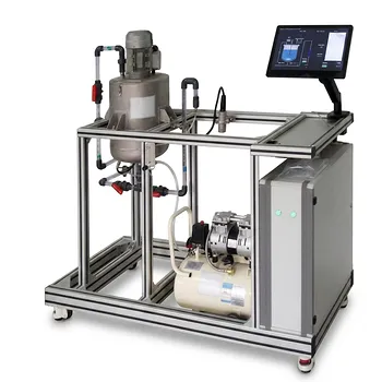
How To Use Stirred Tanks In Series Pilot Plants To Analyze Non-Ideal Flow And Validate Rtd Models.

A pilot plant packed with stirred tanks in series is your laboratory for making invisible mixing flaws visible. Students analyze non-ideal flow by injecting a tracer and recording the outlet concentration over time. From that single experiment, you calculate the Residence Time Distribution (RTD), extract the dimensionless variance, and quantify the equivalent number of perfectly mixed tanks ( N ) or the Peclet number for dispersion. You then superimpose your data onto theoretical models—the tanks‑in‑series ( F(\theta) ) curve, the axial dispersion solution, or the intensity function ( \Lambda(\theta) )—to see exactly where and why real flow deviates from ideal behavior.

Non‑ideal flow is not a nuisance; it is a fingerprint. A cascade of CSTRs in a pilot plant lets you run simple tracer tests, compute model parameters like ( N ) or ( Pe ), and overlay your results on theoretical curves. The moments of mismatch between experiment and theory—early peaks, long tails, shifted means—directly diagnose bypassing, dead zones, and back‑mixing, turning abstract equations into physical insight you can act on.

Turning Tracer Data into a Flow Portrait

Every non‑ideality leaves a signature in the tracer response. To see it, you need a clean stimulus‑response experiment and a structured way to extract the hidden numbers.

The Essential Tracer Experiment

A known amount of tracer (salt, dye, or conductivity‑measuring substance) is introduced at the inlet of your stirred‑tank cascade. A detector at the final outlet records concentration versus time. The raw curve—the ( E(t) ) effluent age distribution—contains all the information about how fluid elements spend their life inside the system.

Calculating the RTD and Its Moments

Convert the concentration‑time data into the normalized ( E(\theta) ) curve using dimensionless time ( \theta = t / \tau ) (where ( \tau ) is the theoretical space time). From ( E(\theta) ) compute the mean residence time and the dimensionless variance ( \sigma_\theta^2 ). These two numbers are the gateway to model validation.

Quantifying Non‑Ideal Flow with Two Classic Models

The dimensionless variance is the Swiss Army knife of RTD analysis. It directly translates into the parameter of your chosen model, letting you replace “looks non‑ideal” with a precise numerical diagnosis.

The Tanks‑in‑Series Model: ( N = 1 / \sigma_\theta^2 )

For a cascade of identical, perfectly mixed tanks, theory says ( \sigma_\theta^2 = 1/N ). Measure your experimental variance, take the reciprocal, and you instantly know the equivalent number of ideal CSTRs that would give your observed spread. A real reactor with ( N = 3.2 ) behaves much closer to a perfectly mixed three‑tank train than to a single tank.

The Axial Dispersion Model: From Variance to Peclet Number

If your pilot plant includes a tubular section or you want to approximate back‑mixing as diffusion‑like dispersion, solve ( \sigma_\theta^2 = \frac{2}{Pe} - \frac{2}{Pe^2}(1 - e^{-Pe}) ) for the Peclet number ( Pe ). A high ( Pe ) means near‑plug flow; a low ( Pe ) signals strong back‑mixing. Comparing the resulting theoretical ( E(\theta) ) curve against your data tests whether dispersion is a reasonable description of your system.

Visual Overlays: Where the Truth Meets the Theory

The real power of a pilot plant comes when you plot the theoretical curves on the same axes as your experimental data. Mismatches are not failures; they are diagnostic tools.

Using the Cumulative ( F(\theta) ) and Intensity ( \Lambda(\theta) )

The cumulative distribution ( F(\theta) ) highlights gross deviations: a curve that rises too early indicates bypassing, while a slow approach to 1.0 points to dead zones. The intensity function ( \Lambda(\theta) )—the conditional exit rate of fluid elements—amplifies subtle differences. If your experimental ( \Lambda(\theta) ) reaches a plateau sooner than the theoretical three‑stirred‑tank curve, you are seeing internal recirculation or short‑circuiting that the ideal model misses.

Direct Comparison with Three Stirred Tanks and 1‑D Diffusion

Plot your pilot‑plant ( F(\theta) ) against the theoretical line for three equal‑volume CSTRs in series. Then overlay the axial dispersion solution with your fitted ( Pe ). The gap between the two theoretical models—and which one hugs your data more tightly—tells you whether the non‑ideality is dominated by back‑mixing between discrete stages or by continuous dispersion down the length.

Reading Flow Malfunctions from the Shape of the E‑Curve

You do not always need heavy‑weight model fitting. A qualitative scan of the ( E(t) ) or ( E(\theta) ) shape itself often flags the main culprit.

Early peak: Short‑circuiting or channeling—fluid sneaks through without mixing.
Long, decaying tail: Stagnant pockets or dead zones slowly release tracer.
Multiple peaks: Parallel flow paths of different velocities or internal recirculation loops.
Shifted mean residence time: The apparent volume is smaller or larger than designed, indicating dead zones or adsorbed tracer.

When students overlay the tanks‑in‑series model and see an early spike that the model cannot reproduce, they immediately grasp why a real stirred tank never behaves like a textbook drawing.

Understanding the Trade‑offs and Limitations

Every experimental method hides assumptions. Recognizing them prevents you from over‑interpreting your data.

The Assumption of Identical Tanks

The simple formula ( N = 1/\sigma_\theta^2 ) assumes all tanks have identical volume and perfect mixing. In a pilot plant, unequal impeller speeds or slightly different vessel geometries introduce extra spread. If you force‑fit an integer ( N ), you may mask a real physical asymmetry.

Sensor Dynamics and Tracer Choice

Conductivity probes, spectrophotometers—their response time and possible adsorption onto walls can distort the late tail of the curve. A late peak may not be a dead zone; it could be measurement lag. Calibrate your sensors and, when possible, deconvolve the instrument response before model validation.

Model Boundaries: When Tanks‑in‑Series Fails

If your actual flow contains strong bypassing or large stagnant regions, the one‑parameter tanks‑in‑series model cannot capture the shape properly. The fitted ( N ) will be low, but the curve’s early hump and long tail will stubbornly refuse to match. That mismatch is itself a valuable lesson: choose a model only after you understand the dominant physical mechanism.

Making the Right Choice for Your Learning Goal

Your approach depends on whether you want to understand the theory, diagnose a real reactor, or prepare for scale‑up.

If your primary focus is building mechanistic understanding: Start with the tanks‑in‑series model. Calculate ( N ) from variance, plot the ( F(\theta) ) curve, and explain why real mixing falls between a single CSTR and plug flow.
If your primary focus is diagnosing plant malfunctions: Use the shape diagnostics first. Look for early peaks, long tails, and split curves, then back them up with the intensity function ( \Lambda(\theta) ) to confirm bypassing or dead zones.
If your primary focus is predicting conversion or selectivity: Fit both the tanks‑in‑series and axial dispersion models, then plug your RTD into the segregated flow model to compute expected conversion. Compare against ideal PFR and CSTR predictions.
If your primary focus is designing a multi‑stage reactor: Map the relationship between the number of physical tanks and the equivalent ( N ). Use that to understand how adding stages narrows the RTD and pushes performance towards plug flow.

The stirred‑tank cascade in your pilot plant is a truth‑telling machine. Give it a tracer, read the signals, and you will never look at a reactor schematic the same way again.

Summary Table:

Flow Phenomenon	E-Curve Signature	Physical Diagnosis
Short-Circuiting	Early, sharp peak	Fluid bypassing the primary mixing zone
Dead Zones	Long, decaying tail	Stagnant pockets slowly releasing tracer
Bypassing/Recirculation	Multiple peaks	Parallel flow paths or internal loops
Volume Mismatch	Shifted mean residence time	Inactive volume or tracer adsorption on walls

Bring Chemical Engineering Theory to Life with LABPARK

Bridge the gap between textbook equations and real-world process dynamics. LABPARK provides advanced Educational and Vocational Unit Operations Pilot Plants in chemical engineering, bioprocess & biotech, and environmental & water treatment designed specifically for universities, research institutes, and enterprises.

Our state-of-the-art pilot plants—including customizable stirred-tank cascades—enable students and researchers to perform precise tracer studies, analyze non-ideal flow, and validate RTD models with industry-grade equipment.

Ready to elevate your engineering lab's capabilities? Contact LABPARK today to discover our range of pilot plant solutions!