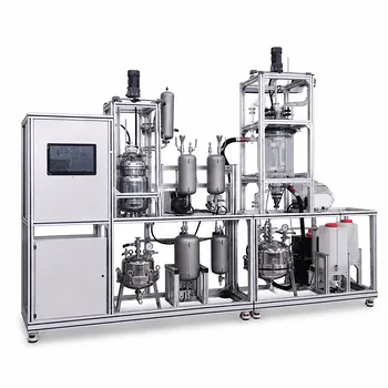
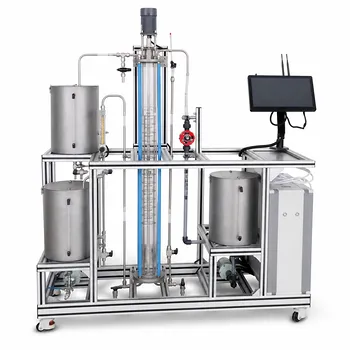
How Can Multi-Stage Solid-Liquid Extraction Pilot Plants Validate Kremser Models? Improve Scale-Up Confidence

Multi-stage solid-liquid extraction pilot plants can validate Kremser-based mass balance models by providing steady-state concentration and flow data from every stage. Researchers operate mixing and separation stages in counter-current or continuous mode, measure soluble-solute concentrations in the entering and leaving liquid and solid streams, and compare the measured concentration profile with the profile predicted by the Kremser equation. The comparison reveals theoretical stage requirements, stage efficiency, model error, and the effect of solvent-to-feed ratio on recovery.

A pilot plant turns the Kremser equation from a theoretical calculation into a testable process model: measured stream balances establish whether the model describes the system, while deviations identify nonideal contact, incomplete separation, equilibrium limitations, or measurement error.

Establishing the Pilot-Plant Basis

Define the Solute and Process Streams

The first step is to identify the soluble component being recovered, such as a dissolved compound in plant pulp, biomass, or another porous solid. The principal streams are the incoming solid feed, extraction solvent, exiting solid or raffinate, and solute-rich liquid extract.

For each stream, measure total flow and solute concentration. Moisture content, solvent retained by the solids, and insoluble carrier mass should also be tracked because they affect the actual mass balance.

Configure Multiple Contact Stages

A suitable pilot plant consists of several mixing tanks followed by separation units. Each tank provides contact between the solid and liquid phases, while screens, filters, centrifuges, or settling devices separate the phases before the next stage.

For counter-current operation, relatively fresh solvent contacts solids that have already undergone extraction, while the most concentrated liquid contacts the incoming solid feed. This arrangement generally provides stronger driving force and more effective solvent use than repeated single-stage batch contact.

Reach and Confirm Steady State

Kremser-based comparisons are meaningful only when the plant has reached a stable operating condition. Researchers should wait until flow rates and solute concentrations at the stage outlets remain acceptably constant over repeated samples.

The operating record should include solvent rate, solid-feed rate, residence time, mixing conditions, temperature, moisture content, and the concentration of each relevant stream. These variables help distinguish model limitations from unstable operation.

Applying the Kremser Equation to Pilot Data

Define the Equilibrium Relationship

The Kremser method requires an equilibrium relationship between solute concentration in the liquid and the corresponding concentration associated with the solid phase. For a simplified system, this relationship may be represented by a linear distribution or partition coefficient.

The assumed relationship must be established from equilibrium experiments or supported by reliable data. If the solid is porous, swelling, chemically reactive, or internally diffusion-limited, a simple linear equilibrium model may describe only part of the operating range.

Use Consistent Flow and Concentration Bases

The model should use consistent solute-free or carrier-free flow rates where appropriate. In solid-liquid systems, the liquid retained in the solids can make the liquid flow rate change from stage to stage, so treating all liquid flows as constant may introduce systematic error.

Researchers should state whether concentrations are expressed as mass fractions, mass ratios, or solute mass per unit carrier. The same basis must be used in the Kremser calculation and in the experimental material balances.

Calculate the Theoretical Stage Requirement

Using the equilibrium parameter, solvent-to-feed ratio, inlet and outlet compositions, and the selected flow assumptions, calculate the number of ideal equilibrium stages required to achieve the measured recovery or raffinate concentration.

The result is a theoretical requirement rather than a direct count of physical tanks. It represents the number of ideal contacts that would be needed if each stage reached the assumed equilibrium state and phase separation were complete.

Compare Predicted and Measured Profiles

The strongest validation does not rely only on final extract or raffinate composition. Measure solute concentrations after each stage and compare the complete experimental concentration profile with the Kremser prediction.

A close profile match supports the equilibrium and flow assumptions. A consistent departure at particular stages can indicate poor mixing, solids bypassing, solvent retention, incomplete separation, or a changing equilibrium relationship.

Quantifying Actual Stage Efficiency

Relate Ideal and Physical Stages

After calculating the ideal stage requirement, compare it with the number of physical contact stages installed in the pilot plant. A plant requiring more physical stages than the theoretical calculation indicates that the stages are not achieving complete equilibrium contact.

An apparent stage efficiency can be estimated by relating the ideal stage performance to the measured performance of the corresponding physical stage. The exact efficiency definition should be stated because overall, Murphree-type, and stagewise effectiveness measures are not interchangeable.

Evaluate Stage-by-Stage Performance

Stage performance may vary across the plant. Incoming solids may be difficult to wet, late-stage solids may retain more liquid, and concentration gradients may produce different extraction driving forces from one stage to another.

Stagewise samples allow researchers to identify where most of the extraction occurs and where additional residence time, mixing, or separation capacity would have the greatest effect.

Test Operating Variables

Repeat the experiments at different solvent-to-feed ratios, flow rates, residence times, temperatures, and mixing intensities. The Kremser model can then be tested across a range of operating conditions rather than against one isolated data point.

Increasing solvent flow may improve recovery and reduce residual solute in the solids, but it can also dilute the extract and increase downstream separation costs. Pilot data make this trade-off measurable.

Verifying the Overall Mass Balance

Close the Solute Balance

For a steady-state system, the solute entering with the solid feed and solvent should approximately equal the solute leaving in the extract, residual solids, retained liquid, and any measured losses:

[ \text{solute in} \approx \text{solute out} ]

The balance should be evaluated for the entire plant and, where possible, around each individual stage. A poor balance closure means that model validation is inconclusive because the measured data do not yet provide a reliable representation of the process.

Close the Carrier and Liquid Balances

Solute balance alone is insufficient. The insoluble solid carrier, solvent, and water or moisture should also be tracked, particularly when solids carry liquid between stages.

Accounting for entrained liquid is essential in counter-current extraction because it changes the effective liquid-to-solid ratio and can transfer dissolved solute independently of the intended stage equilibrium.

Remove Redundant Equations

When stream compositions are represented as mass fractions, all component fractions in a stream must sum to one. Consequently, one component balance may be mathematically dependent on the remaining component balances and the total mass balance.

The model should therefore include only independent equations. Removing redundant balances avoids singular or overdetermined equation systems and makes discrepancies easier to interpret as actual process errors.

Understanding the Trade-offs

Ideal Equilibrium Is Not Guaranteed

The Kremser equation commonly assumes ideal stage contact, a defined equilibrium relationship, and simplified flow behavior. Real solid-liquid stages may be limited by particle diffusion, inadequate wetting, channeling, solids settling, or short-circuiting.

A disagreement between predicted and measured performance does not automatically invalidate the equation. It may show that the pilot plant requires an efficiency correction or a more detailed transport model.

Constant Flow Assumptions Can Fail

Solids may absorb solvent, release moisture, or carry liquid into the next stage. These effects alter the phase flow rates and can invalidate a constant-flow approximation.

For systems with substantial liquid retention or changing moisture content, researchers should use measured stagewise flows or revise the model to include entrainment and phase transfer.

Concentration Measurements Can Mislead

Sampling errors are especially important when solute concentrations are low or when suspended solids remain in the liquid sample. The sample may not represent the separated extract phase, and an unmeasured dissolved fraction may remain with the wet solids.

Samples should be filtered or otherwise prepared consistently, and flow measurements should be taken on the same basis as the concentration measurements.

More Solvent Is Not Always Better

A higher solvent-to-feed ratio can increase extraction driving force and reduce residual solute in the solids. However, it may produce a more dilute extract and increase pumping, solvent recovery, and downstream concentration requirements.

The appropriate operating point is therefore defined by the combined recovery, extract concentration, solvent consumption, and separation cost rather than by recovery alone.

Making the Right Choice for Your Goal

A useful validation program connects the model calculation, the pilot measurements, and the intended scale-up decision.

If your primary focus is model validation: Operate at steady state, measure every stage inlet and outlet, and compare the full concentration profile rather than only the final recovery.
If your primary focus is stage-count design: Use measured equilibrium behavior and solvent-to-feed ratios to calculate theoretical stages, then convert the result to physical stages using experimentally determined efficiency.
If your primary focus is solvent efficiency: Run controlled tests at several solvent-to-feed ratios and evaluate recovery together with extract concentration and solvent consumption.
If your primary focus is scale-up: Close total, solute, solvent, and carrier balances while accounting for liquid retained by solids and nonideal stage behavior.
If your primary focus is equation robustness: Test the Kremser model under different flow rates, residence times, and feed compositions to identify the range in which its assumptions remain valid.

A well-instrumented multi-stage pilot plant makes the Kremser equation an auditable engineering model whose predictions can be accepted, corrected, or replaced on the basis of measured process behavior.

Summary Table:

Validation focus	Key measurements	Engineering insight
Stagewise performance	Inlet and outlet flow rates and solute concentrations	Compares measured profiles with Kremser predictions
Equilibrium behavior	Solid-liquid equilibrium data and distribution parameters	Tests whether model assumptions apply
Stage efficiency	Ideal versus physical stage performance	Converts theoretical stages into practical equipment requirements
Mass balance closure	Solute, carrier, solvent, moisture, and retained-liquid flows	Confirms data reliability and identifies unmeasured losses
Operating trade-offs	Solvent-to-feed ratio, residence time, temperature, and mixing	Balances recovery, extract concentration, and operating cost
Scale-up readiness	Steady-state performance across multiple operating conditions	Defines model limits and supports process design decisions

Planning a solid-liquid extraction process or validating a scale-up model? Contact LABPARK to discuss a pilot plant tailored to your process. LABPARK provides Educational and Vocational Unit Operations Pilot Plants for chemical engineering, bioprocess and biotech, and environmental and water treatment applications. Our systems help universities, research institutes, and enterprises generate reliable stagewise data, evaluate mass balance models such as the Kremser equation, determine practical stage efficiency, and optimize solvent use, recovery, and process performance before full-scale investment.