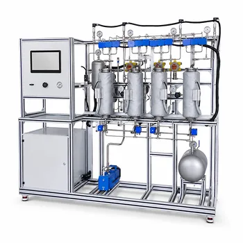
How To Determine Outlet Temperature & Humidity In A Gas Drying Pilot Plant? Lab Guide

The outlet temperature and humidity of a gas drying pilot plant are found by coupling measured inlet data with a mass-and-energy balance and a psychrometric chart. Instructors guide students to first record the inlet gas temperature and dew point—or wet‑bulb temperature—to fix the inlet humidity and specific volume. Next, they calculate mass flow rates of dry gas and moisture. Applying an energy balance that accounts for the evaporation heat of the solvent, the heat capacities of the streams, and any external heat input or loss yields the outlet gas temperature. Finally, the outlet humidity is obtained by adding the evaporated solvent to the inlet moisture load; relative humidity follows from a psychrometric chart or Antoine’s equation. This method transforms the pilot plant into a living textbook of conservation laws.

The real educational power lies in treating the dryer as a conservation‑law boundary. Students who enforce mass and energy balances on the known inlet stream and the solvent’s phase change can predict the outlet gas state before ever looking at a downstream sensor. The calculation not only delivers temperature and humidity but builds a diagnostic intuition for dryer performance that will serve them in design, troubleshooting, and scale‑up.

Setting the Stage: What Students Must Measure

Characterize the Incoming Gas Stream

Students begin by recording the dry‑bulb temperature and dew point of the gas entering the drying chamber.
These two parameters are sufficient to fix the absolute humidity on a psychrometric chart or via the relationship
( H_{in} = 0.622 \frac{p_{v,td}}{p - p_{v,td}} ), where ( p_{v,td} ) is the saturation vapor pressure at the dew‑point temperature.
Knowing the inlet humidity and temperature also gives the specific volume, which is used to convert volumetric airflow readings into a dry‑gas mass flow rate.
Alternatively, if the pilot plant is equipped with a wet‑bulb thermometer, the wet‑bulb temperature together with the dry‑bulb temperature pins the state point just as reliably.

Capture the True Evaporation Load

The mass of solvent leaving the wet material must be measured continuously or at regular intervals.
For batch tray‑drying, students record the decrease in weight of the product over time using the built‑in balance or load cell.
The slope of the weight‑time curve gives the instantaneous drying rate, ( \dot{m}_{evap} ), often expressed in kg·s⁻¹.
When working with a spray or flash dryer that handles liquid feeds, the solvent evaporation rate can be calculated from the feed rate and the measured solids content before and after drying.
This measured evaporation flow is the central bridge between the solid phase and the gas phase.

The Mass Balance Pathway to Outlet Humidity

Start with Inlet Moisture Content

With the inlet absolute humidity ( H_{in} ) and the dry‑gas mass flow rate ( \dot{m}{dry} ), the inlet moisture transport rate is simply ( \dot{m}{dry} \cdot H_{in} ).
This tells students how much water vapor is already present in the air before any drying occurs.

Add the Evaporated Solvent

The mass balance around the dryer states that all evaporated solvent must leave with the exhaust gas:

[ H_{out} = H_{in} + \frac{\dot{m}{evap}}{\dot{m}{dry}} ]

Students compute ( H_{out} ) directly from the measured evaporation rate and the dry‑air flow.
This calculation works equally well for steady‑state continuous processes and for time‑averaged batch experiments, provided the dryer operates under constant inlet conditions.

Locate the Outlet State on the Psychrometric Chart

Once the outlet absolute humidity is known, only one additional independent variable is needed to fix the full thermodynamic state of the exhaust gas.
If the outlet dry‑bulb temperature has been solved via the energy balance (see next section), the intersection of the constant‑temperature line and the constant‑humidity line on the H‑I chart yields the relative humidity, enthalpy, and dew point of the exhaust.
When an online humidity sensor is available, students can verify their mass‑balance humidity against the direct reading—a powerful link between theory and instrumentation.

The Energy Balance to Determine Outlet Temperature

The Governing Equation

The pilot‑plant dryer is an open system where energy is carried in and out by mass flows, exchanged as heat, and consumed for phase change.
A simplified steady‑state energy balance for the gas side can be written as:

[ \dot{m}{dry} , c{p,gas} , (T_{gas,out} - T_{gas,in}) = Q_{ext} - \dot{m}{evap} \Delta H{vap} - \dot{m}{solution} , c{p,solution} , (T_{solution,out} - T_{solution,in}) ]

( Q_{ext} ) represents any intentional heat addition (jacket, preheater) or heat loss to the surroundings.
The term ( \dot{m}{evap} \Delta H{vap} ) is the energy required to vaporize the solvent; for water, use the latent heat at the wet‑bulb temperature.
The solute or wet‑solid stream may enter and leave at different temperatures; students must measure (or estimate) the inlet and outlet solution/solid temperatures to complete the balance.

Solving for the Exhaust Temperature

In many well‑insulated vessels where the wet material remains at the adiabatic saturation (wet‑bulb) temperature during the constant‑rate period, the energy balance simplifies dramatically.
The gas sensible heat lost equals the latent heat gained, so the outlet gas temperature approaches the wet‑bulb temperature of the inlet air.
When external heating or cooling is present, students solve the equation above for ( T_{gas,out} ).
Instructors can ask them to compare the calculated outlet temperature against the reading of a downstream thermocouple—a discrepancy often reveals unaccounted heat losses or incomplete wetting of the solid surface.

Understanding the Trade‑offs and Pitfalls

Where Assumptions Break Down

The elegant mass‑and‑energy method assumes steady‑state operation, negligible heat leaks, and uniform conditions across the dryer cross‑section.
In batch tray dryers, the evaporation rate changes as the material dries; students must either use an average rate over the constant‑rate period or perform a dynamic balance.
The energy balance also assumes that the latent heat of vaporization is supplied exclusively by the gas—a reasonable assumption in a purely convective dryer, but not if the vessel is radiatively heated or if solution pre‑heating contributes significantly.

Measurement Sensitivity and Dew Point Errors

Inlet humidity derived from a dew‑point hygrometer is highly accurate, but a wet‑bulb psychrometer can suffer from poor ventilation or a dried‑out wick.
A 1 °C error in wet‑bulb reading can shift the computed inlet humidity by several percent, which propagates directly into the outlet humidity.
Instructors should therefore emphasize the importance of sensor maintenance and, where possible, use the dry‑bulb/wet‑bulb pair for in‑class demonstrations while cross‑checking with the plant’s built‑in dew‑point sensor.

Condensation: The Invisible Saboteur

If the calculated outlet temperature lies below the dew point of the exhaust air, moisture will condense inside the ducting.
This not only invalidates the downstream humidity measurement but also teaches students a critical industrial lesson: condensation causes product clumping, corrosion, and baghouse blockage.
A pilot plant that visibly sweats inside the exhaust line is an unforgettable reminder to keep process air above the dew point.

Making the Right Choice for Your Instructional Goal

The same pilot plant can serve multiple learning objectives. Tailor the lab approach to match the skill you want students to take away.

If your primary focus is thermodynamic fundamentals: Have students solve the full energy balance and compute the outlet temperature using measured heat capacities and latent heat. This forces deep engagement with enthalpy, phase change, and the psychrometric chart.
If your primary focus is measurement validation and process control: Ask students to record the outlet dry‑bulb and wet‑bulb temperatures directly, then use the mass‑balance humidity and energy‑balance temperature to cross‑check sensor health. The exercise builds confidence in industrial instrumentation.
If your primary focus is scale‑up and dryer design: Combine the outlet‑state calculation with a drying‑rate curve analysis. Students first determine ( H_{out} ) and ( T_{out} ) for the constant‑rate period, then use those values to calculate mass‑transfer coefficients and critical moisture content—direct inputs for sizing full‑scale dryers.

When instructors frame the pilot plant as a set of living equations, students leave the lab not just with numbers but with the intuition that every degree of outlet temperature and every gram of moisture carries a story of mass, energy, and the physics of drying.

Summary Table:

Parameter	Measurement / Method	Core Tool / Equation
Inlet Humidity ($H_{in}$)	Dry-bulb & dew-point (or wet-bulb) temperature	Psychrometric chart / Antoine equation
Evaporation Load ($\dot{m}_{evap}$)	Weight change over time (load cell / balance)	Slope of weight-time curve
Outlet Humidity ($H_{out}$)	Mass balance (inlet moisture + evaporated mass)	$H_{out} = H_{in} + \dot{m}{evap}/\dot{m}{dry}$
Outlet Temp ($T_{out}$)	Energy balance (sensible & latent heat exchange)	Open system energy balance equation

Bring Chemical Engineering Thermodynamics to Life with LABPARK

Bridge the gap between textbook theory and physical reality for your students. LABPARK designs and manufactures high-quality Educational and Vocational Unit Operations Pilot Plants in chemical engineering, bioprocess & biotech, and environmental & water treatment tailored for universities, research institutes, and enterprises.

Our systems are equipped with industrial-grade sensors, enabling students to accurately measure, balance, and scale up processes just like in real-world industries.

Contact our specialists today to find the perfect pilot plant solution for your lab.