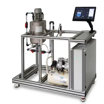
How Are The Physical Features Of Creeping Flow Demonstrated In Chemical Engineering Fluid Mechanics Unit Operations Training Equipment? See Viscous Flow In Action

Creeping flow is demonstrated by making viscous forces overwhelmingly stronger than inertial forces. In chemical engineering fluid mechanics training equipment, this is achieved with very viscous fluids, narrow flow passages, small-scale channels, or slowly moving boundaries that produce Reynolds numbers much less than one. Students then observe three defining features: pseudosteady behavior, kinematic reversibility, and flow behavior governed primarily by viscosity rather than momentum.

Creeping-flow equipment turns an abstract low-Reynolds-number model into observable behavior: the fluid responds essentially immediately to changes, does not coast, and retraces the same flow pattern when the direction of motion is reversed.

How Training Equipment Creates Creeping-Flow Conditions

Using High-Viscosity Fluids

Training systems may use fluids with relatively high dynamic viscosity to reduce the Reynolds number while maintaining a measurable flow rate. Polymer solutions and other viscous working fluids make the effect of viscous resistance readily observable.

The governing dimensionless relationship is:

[ Re=\frac{\rho u L}{\mu} ]

where (\rho) is fluid density, (u) is characteristic velocity, (L) is characteristic length, and (\mu) is dynamic viscosity. Increasing viscosity, reducing velocity, or reducing passage size drives the system toward the creeping-flow regime.

Using Small-Scale Flow Passages

Microchannels, capillary tubes, narrow gaps, and porous media provide the small characteristic dimensions needed for very low Reynolds numbers. These configurations are especially useful because students can study viscous transport without requiring extremely slow operation in a large apparatus.

Controlling Surface or Boundary Motion

Some demonstrations impose motion through a moving wall, plate, or boundary rather than relying only on pressure-driven flow. Reversing the direction of that motion allows students to test whether the flow pattern reverses in the predicted manner.

The Physical Features Students Observe

Pseudosteady Response to Changes

At very low Reynolds numbers, inertial terms in the Navier-Stokes equations become negligible. The flow is therefore described approximately by the linear Stokes relation:

[ \nabla p=\mu\nabla^2\mathbf{v} ]

A change in applied pressure or boundary velocity produces an almost immediate corresponding change in the velocity and pressure fields. The fluid does not continue moving because of stored momentum after the driving force is removed.

Absence of Inertial Coasting

In ordinary flows, fluid momentum can cause acceleration, deceleration, overshoot, or continued motion after a change in operating conditions. Creeping-flow equipment demonstrates that these effects are effectively absent when viscous forces dominate.

Students can compare the observed response with a higher-Reynolds-number system to see that the low-Reynolds-number fluid behaves more like a continuously adjusted viscous medium than a moving mass.

Kinematic Reversibility

The linearity of the Stokes equations produces kinematic reversibility. If the direction of a boundary movement or pressure-driven flow is reversed, the local velocity vectors and streamlines reverse correspondingly.

A particle-tracking setup can make this visible. Particles that move along a particular path during the forward motion should retrace that path when the motion is reversed, provided the experiment remains within the creeping-flow regime.

Viscosity-Dominated Drag

The drag on suspended particles is governed primarily by viscous resistance rather than inertial wake formation. This makes low-Reynolds-number equipment useful for examining particulate settling, particle transport, and suspension behavior.

Students can relate the observed particle motion to suspension-viscosity models and to the drag forces encountered in colloidal and particulate processing.

What Unit Operations Equipment Can Demonstrate

High-Viscosity Flow Modules

A high-viscosity flow module can be used to measure pressure drop, flow rate, and fluid response under controlled conditions. The results demonstrate how strongly viscosity controls resistance to motion when inertial contributions are negligible.

Such a module can also help students connect laboratory observations with polymer melt processing, where high viscosity can place parts of the process near a viscous-dominated flow regime.

Microchannel and Capillary Systems

Microchannel and capillary apparatus provide direct examples of low-Reynolds-number transport in confined geometries. Students can investigate how channel size, viscosity, and pressure difference affect the flow.

These systems are relevant to microfluidic transport and bioprocessing applications, where small dimensions make creeping-flow behavior common.

Particle-Tracking Apparatus

Transparent flow sections containing tracer particles or suspended particles allow students to visualize streamlines and particle trajectories. By changing the pressure gradient or reversing a moving boundary, they can examine reversibility and viscous drag.

The same equipment can support investigations of suspension viscosity, colloid transport, and particulate motion through low-inertia environments.

Porous-Media Demonstrations

Flow through packed beds or other porous media can be operated at sufficiently low velocities for viscous resistance to dominate. Measurements of pressure drop and flow rate then illustrate the relationship between applied pressure and viscous transport through complex passages.

This connects creeping-flow principles to filtration, packed-bed operations, and transport through porous structures.

How the Demonstrations Are Interpreted

Comparing Measured Flow With Reynolds Number

Students should calculate the Reynolds number using the actual fluid properties, characteristic velocity, and equipment dimensions. The visual appearance of smooth flow alone is not enough to establish creeping flow; the operating conditions must support (Re \ll 1).

This calculation links the physical demonstration to the dimensionless analysis used in chemical engineering design.

Relating Pressure to Velocity

Because the Stokes equations are linear, velocity generally changes proportionally with the applied pressure gradient for a fixed geometry and viscosity. A pressure-flow-rate experiment can therefore show the direct relationship expected when inertial losses are negligible.

Departures from this relationship may indicate that the Reynolds number is no longer sufficiently small, that the fluid is non-Newtonian, or that measurement and equipment effects are significant.

Tracking Response After a Change

A step change in pressure or boundary speed can be monitored using flow meters, pressure sensors, or particle imaging. The expected result is a rapid transition to the new flow field without a prolonged inertial transient.

In practice, the equipment and instrumentation may have their own response times. The demonstration therefore shows that fluid inertia is negligible relative to the apparatus response, rather than proving that every physical process is mathematically instantaneous.

Understanding the Trade-offs

The Flow Must Be Slow or Highly Viscous

Achieving (Re \ll 1) often requires high-viscosity fluids, low velocities, small channels, or a combination of these conditions. These restrictions can make experiments slower and may reduce the range of operating conditions available to students.

Reversibility Has Conditions

Flow reversal is an ideal property of creeping flow governed by linear, time-independent equations. It can be disrupted by particle inertia, diffusion, wall roughness, non-Newtonian effects, unsteady operating conditions, or a Reynolds number that is no longer very small.

The demonstration should therefore control the reversal carefully and verify that the relevant low-Reynolds-number assumptions remain valid.

Not All Unsteady Flow Is Creeping Flow

A draining-vessel experiment demonstrates unsteady operation by tracking liquid level and discharge over time. It is useful for teaching dynamic balances and changing hydrostatic head, but it does not automatically demonstrate creeping flow.

The distinction is important: creeping flow concerns the relative importance of inertia and viscosity, whereas unsteady flow concerns whether conditions change with time. A process can be unsteady without being creeping, or creeping with an externally changing pressure or boundary condition.

Equipment Effects Can Mask the Fluid Behavior

Tubing compliance, pump fluctuations, sensor delays, and flow-development regions can affect the measured response. Good laboratory practice compares sensor readings with the expected Stokes-flow scaling and identifies which observed delays belong to the equipment rather than the fluid.

Making the Right Choice for Your Goal

The most effective training setup combines controlled low-Reynolds-number conditions with direct measurement or visualization.

If your primary focus is viscous pressure-flow behavior: Use a high-viscosity flow module or capillary system and compare measured pressure drop with flow rate at (Re \ll 1).
If your primary focus is flow reversibility: Use a transparent channel or moving-boundary apparatus with tracer particles and reverse the driving motion under controlled conditions.
If your primary focus is particle transport: Use particle-tracking equipment to examine viscous drag, suspension motion, and the effect of fluid viscosity.
If your primary focus is microfluidic or porous-media transport: Use narrow channels or packed media and relate pressure-driven flow to the small characteristic length scale.
If your primary focus is unsteady unit operations: Use a draining-vessel system for dynamic mass balances, while treating its time-dependent behavior separately from creeping-flow physics.

When the equipment is operated at sufficiently low Reynolds number, students can directly see that viscosity, rather than inertia, determines how the fluid moves.

Summary Table:

| Training Equipment | Key Demonstration | Main Measurements or Observations |\n|---|---|---|\n| High-viscosity flow module | Viscosity-dominated pressure-flow behavior | Pressure drop, flow rate, Reynolds number |\n| Microchannel or capillary system | Low-Reynolds-number transport in narrow passages | Channel size, pressure, velocity, flow response |\n| Particle-tracking apparatus | Kinematic reversibility and viscous drag | Particle paths, streamline reversal, suspension motion |\n| Packed-bed or porous-media system | Viscous flow through complex passages | Pressure drop, flow rate, permeability relationship |\n| Step-response setup | Pseudosteady behavior with negligible coasting | Response to pressure or boundary-velocity changes |\n| Draining-vessel system | Unsteady operation, separate from creeping flow | Liquid level, discharge, dynamic mass balance |

Need reliable equipment to teach low-Reynolds-number transport clearly? Contact LABPARK to discuss your requirements. LABPARK provides Educational and Vocational Unit Operations Pilot Plants for chemical engineering, bioprocess and biotech, and environmental and water treatment programs. Our universities, research institutes, and enterprise customers can use high-viscosity flow modules, capillary and microchannel systems, particle-tracking equipment, and porous-media units to connect Reynolds-number analysis with measurable pressure-flow data, particle motion, reversibility, and real process applications. We can help you select a practical configuration, match the system to your curriculum or research goals, and create hands-on training that strengthens engineering analysis and process understanding.