Why Is Trial-And-Error Necessary For Fluid Flow Rate? Iterative Calculation Steps Explained

Here’s the direct answer: the trial-and-error method is unavoidable because the two critical variables—flow velocity and friction factor—form a circular dependency through the Reynolds number. You simply cannot solve for one without already knowing the other, so an iterative approach is the standard engineering workaround.

Fluid flow problems where both velocity and friction factor are unknown force you into a loop. You guess a friction factor to break the cycle, calculate a velocity, check if the guess was right, and repeat until the numbers stabilize. This isn’t a flaw in the math—it’s a natural consequence of how turbulence, pipe roughness, and fluid properties interact. Training systems use this exact loop to build the judgment engineers need for real-world piping design.

The Unavoidable Circular Dependency

The root of the trial-and-error necessity is the relationship between head loss, velocity, and friction factor. The Darcy–Weisbach equation ties head loss directly to ( f \cdot V^2 ), but ( f ) itself is not a constant—it’s a function of the Reynolds number, ( Re ), and relative roughness.

Two Unknowns, One Equation

When you know the head loss and pipe geometry but need the flow rate, you face a single equation with two unknowns: velocity ( V ) and friction factor ( f ). You cannot isolate either variable because ( f ) depends on ( Re = \rho V D / \mu ), which contains ( V ). The moment you try to solve directly, you’re chasing your own tail.

Why the Reynolds Number Creates the Loop

The Moody chart (or the Colebrook equation) makes ( f ) a non-linear function of ( Re ). In the transitional and fully rough turbulent zones, ( f ) changes with ( Re ) in ways that defy a closed-form solution. So any attempt at a direct algebraic answer fails. You must invoke an iterative scheme that leverages the fact that ( f ) varies more slowly than ( V ), allowing successive guesses to converge.

How the Trial-and-Error Method Works in Practice

Training systems replicate the exact sequence a professional engineer follows. The process is structured around a clear, repeatable loop that teaches discipline and exposes the sensitivity of the result to the initial guess.

Step 1: Assume an Initial Friction Factor

You start by picking a first guess for ( f ). The safest, most common assumption comes from the fully turbulent region of the Moody chart, where the friction factor depends only on the pipe’s relative roughness ( \varepsilon/D ). This guess is intentionally conservative, often higher than the true ( f ), which makes the subsequent velocity calculation a safe low estimate.

Step 2: Calculate a Trial Velocity

With the guessed ( f ), you solve the Darcy–Weisbach equation for ( V ): [ V = \sqrt{ \frac{2 g D h_f}{f L} } ] This gives you a first number for the fluid speed. It’s not yet correct—it’s just a stepping stone.

Step 3: Compute the Reynolds Number and Refine ( f )

Plug that trial velocity into ( Re = \rho V D / \mu ). Now you have a concrete Reynolds number. You then revisit the Moody chart or the Colebrook equation to extract a new friction factor ( f_{\text{new}} ) corresponding to this ( Re ) and the pipe’s roughness.

Step 4: Iterate Until Convergence

Compare ( f_{\text{new}} ) with your previous guess. If the difference exceeds a set tolerance—typically 3%—you set the guessed ( f ) equal to ( f_{\text{new}} ) and repeat from Step 2. The loop continues until successive values of ( f ) stop moving meaningfully. At that point, you know you’ve found the operating point where the friction factor and velocity are mutually consistent.

Why Training Systems Prioritize This Method

A fluid transport training system isn’t just about getting an answer; it’s about embedding the logic of iterative solution into a student’s workflow. The hardware and curriculum together make the hidden loop visible.

From Manual Calculation to Visual Intuition

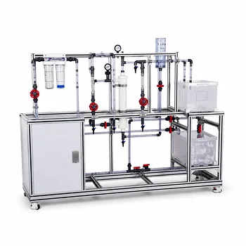
Supplementary references highlight how an experimental pilot plant lets students bypass tedious manual iterations by directly measuring pressure drops and flow rates for different pipes. When these data points are plotted on a Moody diagram, the transition from laminar to turbulent flow becomes a visual story. Students see not just a number, but a pattern—why the friction factor soars after the critical Reynolds number and how roughness dominates in the fully turbulent zone.

Building Engineering Judgment for Non-Linear Problems

The trial-and-error exercise teaches a vital lesson: many real problems in fluid dynamics have no neat formula. It forces the mind to think in terms of convergence, stability, and initial guess sensitivity. An engineer who has walked through this loop manually is less likely to blindly trust a software solver and more likely to recognize when an answer violates physical intuition.

Understanding the Trade-offs and Pitfalls

No method is flawless. The trial-and-error approach has limitations that training systems deliberately expose to prevent overconfidence.

Convergence Is Not Guaranteed for All Scenarios

In most practical pipe-flow cases, the method converges quickly because ( f ) varies gently. However, if you start with a wildly unrealistic guess in the laminar zone for a turbulent-flow problem (or vice versa), the loop may need many more steps—or even diverge if the solver loses physical bounds. Training systems typically guide students to use the fully turbulent assumption precisely to avoid this instability.

The 3% Tolerance Is a Practical, Not Absolute, Threshold

The typical 3% tolerance is an engineering convention. It reflects the fact that friction factor correlations themselves have inherent uncertainty (the Colebrook equation is empirical, accurate to about 10–15%). Pushing for tighter convergence wastes time without meaningfully improving the real-world accuracy of the flow rate estimate.

Overlooking the Educational Value of the Struggle

A common pitfall is seeing the iterative process as mere busywork. The actual deep need is to internalize the coupling between velocity and energy loss. A student who runs a manual trial-and-error once will forever understand why pump sizing requires an iterative balance between the system curve and the pump curve.

Making the Right Choice for Your Learning or Design Goal

Your path through this material changes depending on whether you’re building fundamental intuition or solving a real-world design problem.

If your primary focus is mastering the physical principles: Spend time with the manual trial-and-error cycle using a Moody chart. Plot your own points from experimental data. The goal is to feel the dependency, not just calculate it.
If your primary focus is efficient piping design: Understand why the loop exists, then rely on validated software or explicit approximations (like the Swamee–Jain equation) that wrap the iteration inside a proven algorithm. Always spot-check a few critical points manually.
If your primary focus is teaching or curriculum design: Integrate the experimental pilot plant observations directly after the manual exercise. Have learners compare their iterative solution to the measured data and discuss the gap—this bridges theory and practice powerfully.

The trial-and-error method isn’t a relic; it’s the clearest window into why pipe flow behaves the way it does. Once you’ve worked through the loop, you’ll never see friction factor as just a number on a chart again.

Summary Table:

Step	Action	Key Details / Formula
1. Assume	Pick initial friction factor ($f$)	Assume fully turbulent region based on relative roughness ($\varepsilon/D$)
2. Calculate	Find trial velocity ($V$)	Solve Darcy-Weisbach equation: $V = \sqrt{2 g D h_f / (f L)}$
3. Compute	Find Reynolds number ($Re$) & new $f$	Calculate $Re = \rho V D / \mu$ and update $f$ using the Moody chart
4. Iterate	Compare $f$ values and repeat	Repeat steps 2 and 3 until the change in $f$ is within 3% tolerance

Bridge Fluid Dynamics Theory and Hands-On Practice

Mastering manual iterative calculations is only the first step. To truly build engineering judgment, students need to see these principles in action.

LABPARK provides state-of-the-art Educational and Vocational Unit Operations Pilot Plants in chemical engineering, bioprocess & biotech, and environmental & water treatment. Specifically designed for universities, research institutes, and enterprises, our systems turn complex math into intuitive, visual physical experiments.

Ready to elevate your engineering curriculum or research facilities? Contact LABPARK today to discover our custom pilot plant solutions!