How To Use Mccabe-Thiele For Liquid-Liquid Extraction: Step-By-Step Parameter Design

The McCabe-Thiele diagram remains the sharpest, fastest tool for translating your separation target into real operating parameters—no simulation package required.
The procedure is straightforward: first you plot the liquid-liquid equilibrium curve (solute weight fraction in the raffinate phase versus the solvent phase). Next, you construct the operating line from overall and component mass balances, fixing the terminal concentrations and the solvent-to-feed ratio. Finally, you step off the theoretical stages between the operating line and the equilibrium curve. That stage count, together with your chosen solvent rate, directly determines the column height, diameter, and the type of extraction equipment needed.

The McCabe-Thiele method solves two problems simultaneously: it finds the minimum solvent rate that makes your separation thermodynamically possible, and it counts the number of ideal contacting stages required. By comparing those stages to the physical height of a pilot column, you get the Height Equivalent to a Theoretical Plate (HETP) or the overall efficiency—turning a graph into a deliverable design.

The Fundamentals of McCabe-Thiele for Liquid-Liquid Extraction

Why a Graphical Method Still Matters

Even with modern process simulators, the McCabe-Thiele plot gives you instant, visible insight into the trade-off between solvent usage and column size.
It forces you to think in terms of equilibrium limits and mass balance constraints—the two absolute boundaries of any extraction.

What the Diagram Represents

The diagram uses two axes:

X-axis: weight percentage (or mass fraction) of solute in the raffinate phase (the feed liquid being depleted).
Y-axis: weight percentage of the same solute in the extract (solvent) phase.

A single point on the equilibrium curve tells you the extract composition that would theoretically be in equilibrium with a given raffinate composition.

Building the Equilibrium Curve

Data Sources and Units

You need experimental ternary equilibrium data for your specific system at the operating temperature.
The primary reference plots weight percentage in the solvent phase (Y) against weight percentage in the feed-raffinate phase (X)—a direct and practical format.

Plotting the Curve

Plot every tie-line endpoint as a (X, Y) pair.
Because extraction equilibrium is rarely a straight line, you will usually see a curved relationship, especially near the origin.

Constructing the Operating Line from Mass Balances

The Overall Material Balance

Under countercurrent flow, you write a solute mass balance over a section of the column.
For a given feed rate, feed composition, and a desired raffinate target composition, the mass balance fixes the relationship between the extract composition and the raffinate composition at every horizontal cross-section.
This relationship is the operating line.

Determining the Solvent-to-Feed Ratio

The operating line’s slope equals the mass ratio of raffinate flow to solvent flow (R/S).
You establish the minimum solvent rate by drawing the steepest possible operating line that just touches the equilibrium curve at the feed end (the “pinch” point).
In practice, you then select a solvent rate about 20–50% above that minimum to avoid an infinite number of stages.

Plotting the Line

Start at the known terminal point: the raffinate exit composition (xR) and the inlet solvent composition (y0)—often pure solvent, so y0 = 0.
The other end of the operating line corresponds to your feed composition (xF) and the exiting extract composition that satisfies the overall mass balance.
Connect those points, and you have a working operating line.

Stepping Off Theoretical Stages

The Step-by-Step Procedure

Begin at the raffinate outlet (xR, y0).
Move vertically up to the operating line, then horizontally left to the equilibrium curve. This first step gives you the first stage’s raffinate composition.
From that equilibrium point, drop vertically to the operating line again, then move horizontally to the equilibrium curve for the next stage.
Repeat until the horizontal step crosses or reaches your feed composition (xF).
Count each horizontal move from the operating line to the equilibrium curve as one theoretical stage.

Connecting to Real Equipment

The number of theoretical stages is ideal—real contactors never reach 100% efficiency.
By measuring the actual packed height or number of physical trays in a pilot column that achieves the same separation, you calculate:

HETP = (packing height) / (theoretical stages)

Overall column efficiency = (theoretical stages) / (actual stages).

This is how the diagram moves from theory to a hardware specification.

Translating the Diagram into Operating Parameters

Solvent Rate and Column Diameter

Your selected solvent rate (derived from the operating line’s slope) fixes the total liquid throughput.
Together with the phase viscosities and density difference, this throughput sets the column diameter via hydraulic flooding correlations.

Column Height and Number of Actual Stages

Once you have the theoretical stage count and the HETP from pilot data or vendor know-how, the required packed height is simply:
Packing height = theoretical stages × HETP.
If you use tray columns, the number of actual trays is theoretical stages divided by tray efficiency.

Equipment Selection Implications

The stage count from McCabe-Thiele feeds directly into equipment choices:

Few stages (1–3): a simple gravity column (packed or plate) often suffices.
Many stages (5+): vertical columns are preferred to save floor space, and you may need mechanical agitation or pulsing for adequate mass transfer.
Ultra-short contact time or emulsion-prone liquids: the stage count and residence-time constraints will push you toward centrifugal extractors.

Understanding the Limitations

The Assumption of Constant Molar Overflow

Classical McCabe-Thiele assumes the raffinate and extract stream flow rates are constant along the column.
When a large fraction of solute transfers, these flow rates change noticeably, and a more rigorous ternary diagram or a corrected operating line may be required for accuracy.

Single-Solute Scope

The method works beautifully for a single transferring solute.
If you are extracting multiple components simultaneously, a single equilibrium curve cannot capture the interactions, and you must move to a full ternary or simulation approach.

Efficiency Is a Moving Target

The theoretical stage count is only as useful as your HETP or efficiency data.
These numbers vary with phase flow rates, packing type, and even trace impurities—the diagram won’t tell you that.

The Trade-off Between Size and Solvent Use

A gentle operating slope (low solvent-to-feed ratio) gives you fewer stages but larger solvent circulation and higher regeneration costs.
A steeper slope (more solvent) reduces the number of stages but increases the column diameter and downstream solvent-recovery burden.
The diagram makes this tug-of-war instantly visible.

How to Apply This to Your Project

The McCabe-Thiele procedure is not a one-size-fits-all recipe; its leverage depends on what you are trying to accomplish.
Tailor your approach like this:

If your primary focus is rapid process screening: Use the diagram to estimate minimum solvent rate and stage count from just the feed and target compositions—it’s an order of magnitude faster than building a full simulation.
If your primary focus is pilot-scale column design: Generate the equilibrium curve from lab shake-flask tests, step off the theoretical stages, and then run the pilot to measure HETP directly. That value scales your production column proportionally.
If your primary focus is troubleshooting an existing unit: Sample the actual raffinate and extract streams, overplot the operating line, and look for pinch points. If the operating line hugs the equilibrium curve, you are operating too close to minimum solvent rate or you have lost packing efficiency.
If your primary focus is equipment selection: Let the stage number drive your decision. One to three theoretical stages from the diagram? A simple packed column will work. Five or more? You are in the territory of mechanically agitated or pulsed columns, and the diagram tells you that from the outset.

Mastering McCabe-Thiele for extraction means you never guess at solvent rates or column heights again—you let the equilibrium and the mass balance draw the line for you.

Summary Table:

Parameter / Step	McCabe-Thiele Graphic Action	Physical Design Implication
Solvent-to-Feed (R/S) Ratio	Slope of the operating line	Determines total liquid throughput and column diameter
Theoretical Stages	Stepping between equilibrium and operating lines	Sets the basis for column height and tray/packing design
Minimum Solvent Rate	Finding the operating line slope at the "pinch" point	Defines the thermodynamic limit; actual rate is usually 1.2–1.5x minimum
HETP & Stage Efficiency	Ratio of physical column height to theoretical stages	Translates graphical stages into actual physical packing height

Scale Up Your Extraction Experiments with LABPARK

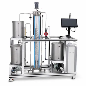
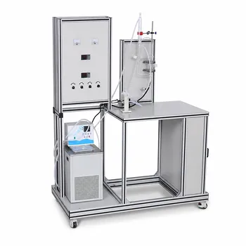
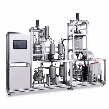
Transitioning from McCabe-Thiele calculations to physical validation requires precise, reliable equipment. LABPARK provides premium Educational and Vocational Unit Operations Pilot Plants in chemical engineering, bioprocess & biotech, and environmental & water treatment. Specifically designed for universities, research institutes, and enterprises, our pilot plants allow you to accurately measure HETP, analyze stage efficiencies, and train the next generation of engineers.

Ready to elevate your laboratory or pilot plant capabilities? Contact LABPARK today to find the perfect system for your needs!