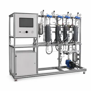
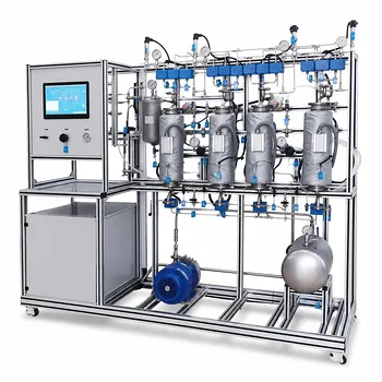
Proportional control usually preserves the second-order nature of a training system while making its response faster and less damped. As proportional gain (K_c) increases, the effective damping factor decreases according to (\zeta'=\zeta/\sqrt{1+K_pK_c}), while the time-scale parameter decreases according to (\tau'=\tau/\sqrt{1+K_pK_c}). The system may therefore develop overshoot and oscillation, although reduced damping alone does not automatically mean instability.
Proportional feedback changes the transient behavior more than the system order: higher gain shortens the response time but reduces damping, narrowing the margin between a well-behaved response and sustained or unstable oscillation.
How Proportional Control Changes the Closed-Loop System
The system remains second-order
Applying proportional feedback to a second-order process does not normally increase its order. The closed-loop response continues to be described by a second-order characteristic equation, with the proportional gain changing its coefficients.
For multi-tank liquid systems or multi-stage thermal units, this means the same basic dynamic structure remains visible during laboratory experiments. The observed changes are primarily in speed, overshoot, and oscillatory behavior.
The response becomes faster
The closed-loop time-scale parameter is represented in the reference model as
[ \tau'=\frac{\tau}{\sqrt{1+K_pK_c}}. ]
As (K_c) increases, (\tau') decreases. The system can respond more quickly to an input or disturbance, but a faster response is not automatically a better response if it produces excessive overshoot or oscillation.
Effective damping decreases
The effective damping factor is
[ \zeta'=\frac{\zeta}{\sqrt{1+K_pK_c}}. ]
With increasing proportional gain, the denominator becomes larger and the effective damping factor becomes smaller. Physically, the response loses some of the natural resistance that suppresses overshoot and oscillation.
What This Means for Stability
High gain can create oscillatory behavior
An open-loop process that is naturally overdamped, with (\zeta>1), may become underdamped after proportional feedback is applied. This occurs when the gain is large enough that
[ \zeta' < 1. ]
The resulting response may contain overshoot and decaying oscillations rather than approaching its target monotonically.
Reduced damping is not the same as instability
A system is underdamped when it oscillates with decreasing amplitude, but it can still be stable. Instability occurs when the oscillations fail to decay or grow over time.
Therefore, increasing (K_c) should be understood as reducing the stability margin and damping quality, rather than as guaranteeing immediate instability. The exact stability boundary depends on the complete process and feedback model.
Stability becomes more sensitive to tuning
At low proportional gain, the process may respond slowly but smoothly. At higher gain, small modeling errors, measurement delays, actuator limitations, or unmodeled dynamics can have a greater effect on the response.
This is why a gain that appears acceptable in a simplified model may produce sustained oscillation or poor behavior on physical training equipment.
What Students Can Observe in the Laboratory
Low proportional gain
The system typically shows a relatively smooth response with limited overshoot. The main drawback is that the response may be slow and may not correct deviations aggressively.
Moderate proportional gain
The process responds more quickly, and tracking or disturbance rejection generally improves. Some overshoot may appear as the reduction in damping begins to affect the transient response.
Excessive proportional gain
The response can become strongly oscillatory, with large overshoot and repeated cycling around the setpoint. If the effective damping becomes sufficiently small, the system approaches a stability boundary and may become difficult to control reliably.
Understanding the Trade-offs
Speed versus damping
Higher proportional gain reduces the modeled time-scale parameter, so the system can reach its target faster. The same gain increase also reduces effective damping, creating more overshoot and oscillation.
The practical objective is therefore not to maximize (K_c), but to select a gain that provides adequate speed while retaining acceptable damping.
Simplicity versus performance
Proportional control is straightforward to implement and makes the relationship between gain and transient response easy to demonstrate. However, proportional action alone may not provide the best compromise between response speed, overshoot, robustness, and steady-state accuracy.
Model prediction versus physical behavior
The second-order model is useful for teaching fundamental dynamics and tuning limitations. Real equipment may include sensor filtering, actuator saturation, dead time, nonlinear flow behavior, thermal losses, and other effects that are not captured by the simplified equations.
These additional effects can make the real stability boundary different from the idealized prediction.
Making the Right Choice for Your Goal
Use the measured response and the complete process model when selecting proportional gain.
- If your primary focus is fast response: Increase (K_c) carefully, monitoring (\tau'), overshoot, and oscillation as the response becomes quicker.
- If your primary focus is stable, well-damped operation: Use a more conservative (K_c) that keeps (\zeta') sufficiently high to prevent excessive oscillation.
- If your primary focus is demonstrating control limitations: Start with an overdamped process and increase (K_c) until the transition toward underdamped behavior is clearly observable.
- If your primary focus is reliable physical equipment operation: Validate the predicted gain on the actual unit while accounting for delays, saturation, measurement noise, and unmodeled dynamics.
Proportional control can make a second-order training system faster, but dependable operation requires preserving enough damping to keep the response controlled.
Summary Table:
| Proportional gain | Response speed | Damping and stability | Typical observation |
|---|---|---|---|
| Low | Slow | Well damped and stable | Smooth response with limited overshoot |
| Moderate | Faster | Reduced damping; generally stable | Improved tracking with some overshoot |
| High | Very fast | Low damping; smaller stability margin | Strong oscillation and large overshoot |
| Excessive | Unreliable | May approach or cross the stability boundary | Sustained oscillation or unstable behavior |
| Key relationship | Effect of increasing gain |
|---|---|
Effective time scale, τ' = τ/√(1 + KpKc) |
Decreases, producing a faster response |
Effective damping, ζ' = ζ/√(1 + KpKc) |
Decreases, increasing overshoot and oscillation risk |
| System order | Normally remains second-order |
| Practical tuning | Balance response speed with damping, delays, saturation, and model uncertainty |
Need a practical way to demonstrate proportional-control tuning and stability limits? Contact LABPARK to discuss Educational and Vocational Unit Operations Pilot Plants for chemical engineering, bioprocess and biotech, or environmental and water treatment applications. LABPARK helps universities, research institutes, and enterprises evaluate response speed, damping, overshoot, and oscillation on hands-on training systems. Our configurable pilot plants support realistic experiments, student instruction, process-development research, controller evaluation, and reliable operator training using equipment that exposes the difference between ideal models and physical process behavior.
Related Products
- Bench Scale Carbon Dioxide Capture Educational Unit Operations Pilot Plant
- Multi Pump Fluid Transport Process Piping Unit Operations Training Pilot Plant
- Electrolyte Distillation Purification and Formulation Educational Pilot Plant
- Multi-Modal Distillation Unit Operations Training Pilot Plant
- Chemical Pipeline Assembly and Fluid Transport Practical Training Unit Operations Pilot Plant
People Also Ask
- What unit operations are critical for CCUS training pilot plants? Build hands-on engineering expertise.
- What are the differences between post- and pre-combustion carbon capture training pilot plants?
- How can pilot plants show tail gas vs flue gas CO2 capture differences? Key educational insights.
- How do temperature variations affect CO2 transport models in pilot plants? Model vs Reality
- How does operating pressure influence the transition between absorption and desorption in a CO2 pilot plant?