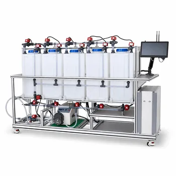
What Are Benchmark Examples Of Second-Order Reactions And How Do They Differ From Zero-Order Kinetics? Compare Pilot-Unit Data

The clearest educational benchmarks are saponification of ethyl acetate and the reaction of ethylene bromide with potassium iodide. Both are commonly treated as bimolecular, second-order reactions, whereas a zero-order reaction has a rate independent of reactant concentration. This difference changes the integrated rate equation, rate-constant units, half-life behavior, and the way students interpret batch or continuous pilot-unit data.

Second-order reactions slow as reactants are consumed; zero-order reactions proceed at a constant rate as long as the zero-order regime remains valid. In an educational pilot unit, this contrast demonstrates how concentration dependence affects reaction-time prediction, reactor sizing, and kinetic-data analysis.

Benchmark Second-Order Reactions in Educational Pilot Units

Saponification of ethyl acetate

The standard example is the alkaline hydrolysis, or saponification, of ethyl acetate:

[ \mathrm{CH_3COOC_2H_5 + OH^- \rightarrow CH_3COO^- + C_2H_5OH} ]

The reaction is commonly modeled as:

[ -r_A = k C_{\text{ester}} C_{\text{OH}^-} ]

This is a second-order rate law overall, because the rate depends on the concentration of two reactants.

When ethyl acetate and hydroxide are introduced at equal initial concentrations and react in a 1:1 stoichiometric ratio, their concentrations remain equal during the reaction. The rate expression then simplifies to:

[ -r_A = k C_A^2 ]

Conductivity as a teaching measurement

Saponification is especially useful in teaching pilot units because its progress can be followed using electrical conductivity.

Highly conductive hydroxide ions are consumed and replaced by acetate ions, which have lower molar conductivity. The resulting decrease in conductivity provides an indirect measurement of reactant conversion.

Students can compare the initial conductivity, the conductivity at time (t), and the final conductivity after effectively complete reaction. These measurements can be converted into concentration or conversion data for determining the second-order rate constant.

Reaction of ethylene bromide and potassium iodide

A second benchmark is the reaction between ethylene bromide and potassium iodide in approximately 99% methanol.

It is used as an example of a bimolecular reaction because the rate depends on the interaction of the two reacting species. In a simplified kinetic treatment, the rate is represented as:

[ -r_A = k C_A C_B ]

If the reactants are prepared at equal initial concentrations, the expression can again reduce to an equal-concentration second-order form proportional to (C_A^2).

This experiment complements the saponification system by showing that second-order behavior is not limited to aqueous ionic reactions.

How Second-Order Kinetics Differ from Zero-Order Kinetics

Rate dependence on concentration

For a second-order reaction involving two reactants:

[ -r_A = k C_A C_B ]

The reaction rate decreases as either reactant is consumed. If both concentrations decrease substantially, the rate can fall sharply during a batch experiment.

For an equal-concentration second-order reaction:

[ -r_A = k C_A^2 ]

The squared concentration dependence makes the rate particularly sensitive to changes in concentration.

For a zero-order reaction:

[ -r_A = -\frac{dC_A}{dt}=k ]

The rate is independent of reactant concentration within the operating range where the zero-order approximation applies.

Integrated batch-reactor equations

For an equal-concentration second-order reaction:

[ \frac{1}{C_A}-\frac{1}{C_{A0}}=kt ]

Using conversion (X_A), the same relationship can be written as:

[ \frac{X_A}{C_{A0}(1-X_A)}=kt ]

The reciprocal concentration therefore varies linearly with time for this second-order model.

For a zero-order reaction:

[ C_{A0}-C_A=kt ]

or:

[ C_{A0}X_A=kt ]

Here, the concentration consumed increases linearly with time. A plot of (C_{A0}-C_A) against (t) should be linear, with slope (k).

Rate-constant units

The units provide a useful diagnostic distinction.

For a second-order rate law:

[ k \sim \frac{\text{volume}}{\text{amount}\cdot\text{time}} ]

For a zero-order rate law:

[ k \sim \frac{\text{amount}}{\text{volume}\cdot\text{time}} ]

In laboratory units, these may appear as (\mathrm{L,mol^{-1},time^{-1}}) for a second-order constant and (\mathrm{mol,L^{-1},time^{-1}}) for a zero-order constant.

Half-life behavior

For an equal-concentration second-order reaction:

[ t_{1/2}=\frac{1}{kC_{A0}} ]

The half-life decreases when the initial concentration increases.

For a zero-order reaction:

[ t_{1/2}=\frac{C_{A0}}{2k} ]

The zero-order half-life increases with initial concentration. This is an important teaching contrast: the second-order half-life is inversely proportional to initial concentration, while the zero-order half-life is directly proportional to it.

What Students Learn from Pilot-Unit Comparisons

Concentration affects reactor time differently

In a second-order batch reaction, the initial stage can be relatively fast because reactant concentrations are high. The reaction then slows progressively as the concentrations fall.

In a zero-order batch reaction, the concentration decreases at a constant rate. The time required to consume a specified concentration interval is therefore constant for a given (k).

Reactor sizing depends on the kinetic model

The kinetic expression determines how much reactor volume or residence time is required to reach a target conversion.

A second-order model predicts increasing difficulty in achieving additional conversion because the reaction becomes slower at lower concentration. A zero-order model predicts a linear relationship between concentration change and processing time within the valid kinetic regime.

Data plots reveal the likely reaction order

For saponification or another equal-concentration second-order system, students can test linearity by plotting:

[ \frac{1}{C_A} \quad \text{against} \quad t ]

For a zero-order system, they can plot:

[ C_{A0}-C_A \quad \text{against} \quad t ]

The plot that gives the stronger linear relationship supports the corresponding kinetic model, although temperature control, mixing, measurement error, and concentration calibration must also be considered.

Understanding the Trade-offs

A second-order model may depend on stoichiometric conditions

The simplified equation ( -r_A=kC_A^2 ) applies most directly when the two reactants have equal initial concentrations and react in equal stoichiometric proportions.

If the initial concentrations are unequal, the more general expression ( -r_A=kC_A C_B ) should be retained. Treating every bimolecular reaction as (kC_A^2) can produce an incorrect rate constant.

Zero-order behavior is usually a regime, not a universal mechanism

Zero-order kinetics often describe a condition in which the controlling reactive sites or another rate-limiting feature are saturated. For example, heterogeneous catalytic surfaces can become saturated, making further increases in reactant concentration ineffective over a particular operating range.

This does not mean the reaction is concentration-independent under all temperatures, pressures, or compositions. Pilot-unit data should be checked for the range over which the zero-order approximation remains valid.

Apparent order can change with operating conditions

Non-elementary reactions can exhibit different apparent orders in different concentration regimes. Active intermediates, deactivation, or competing steps can cause a reaction to appear second-order at low concentration and closer to first-order at high concentration.

Students should therefore distinguish an experimentally observed apparent reaction order from a universal mechanistic statement.

Conductivity requires careful interpretation

Conductivity is a practical online measurement for saponification, but it is an indirect concentration measurement. The relationship between conductivity and concentration must be established consistently, and the initial and final conductivity values must be measured reliably.

Temperature variation is also important because conductivity is temperature-sensitive. Poor mixing or sensor placement can introduce additional error into the inferred kinetics.

How to Apply This to Your Project

Use the kinetic model that matches both the reaction chemistry and the experimental data.

If your primary focus is demonstrating second-order kinetics: Use ethyl acetate saponification or ethylene bromide–potassium iodide, monitor concentration or conductivity over time, and test a reciprocal-concentration plot for linearity.
If your primary focus is demonstrating zero-order kinetics: Plot (C_{A0}-C_A) against time and verify that the slope is approximately constant over the selected operating range.
If your primary focus is reactor sizing: Use the integrated rate equation appropriate to the verified reaction order rather than assuming that all batch reactions have constant rates.
If your primary focus is comparing pilot-unit experiments: Keep temperature, mixing, initial concentrations, and measurement methods controlled so that differences in concentration dependence are not confused with equipment effects.

Understanding whether the rate decreases with concentration or remains constant is the foundation for interpreting reaction-time data and designing reliable educational pilot-unit experiments.

Summary Table:

Feature	Second-order reaction	Zero-order reaction
Benchmark	Ethyl acetate saponification; ethylene bromide with potassium iodide	Saturated or rate-limited reaction regime
Rate law	-rA = kCA CB; often -rA = kCA^2 for equal concentrations	-rA = k
Batch relationship	1/CA - 1/CA0 = kt	CA0 - CA = kt
Rate behavior	Slows as reactants are consumed	Remains constant within the valid regime
Rate-constant units	Volume/(amount x time), such as L mol-1 time-1	Amount/(volume x time), such as mol L-1 time-1
Half-life	t1/2 = 1/(kCA0); decreases as initial concentration rises	t1/2 = CA0/(2k); increases as initial concentration rises
Recommended data plot	1/CA versus time	CA0 - CA versus time
Teaching measurement	Conductivity can track hydroxide consumption during saponification	Concentration measurements should confirm a constant-rate regime

Planning an educational reaction engineering laboratory or pilot unit? Contact LABPARK to discuss your requirements. LABPARK provides Educational and Vocational Unit Operations Pilot Plants for chemical engineering, bioprocess and biotechnology, and environmental and water treatment applications. Our systems help universities, research institutes, and enterprises teach and validate reaction kinetics through controlled batch or continuous experiments, concentration and conductivity measurements, reactor-sizing studies, and repeatable data analysis. We can help you select a configuration for demonstrating second-order and zero-order behavior, match instrumentation to your curriculum or research goals, and develop a practical pilot-unit solution for reliable training and process evaluation.