The draining of a process vessel is far more than a simple batch operation—it is a masterclass in transient systems thinking. In chemical engineering unit operations training, unsteady-state flow is analyzed by coupling a dynamic mass balance with the instantaneous Bernoulli equation. Students derive a differential equation that relates the falling liquid level to the discharge velocity, integrate it to predict draining time or liquid height, and then verify their model by measuring the actual level change in a graduated pilot-plant vessel over time. This hands-on approach transforms an abstract mathematical concept into a tangible, experimentally validated skill.
The true power of this exercise lies in its integration of first-principles modeling with live data acquisition. It teaches that even a simple draining tank is a time-dependent system, where the instantaneous velocity depends on the height, which itself is constantly changing—a recurring theme in process dynamics and control.
The Core Analytical Framework
The analysis rests on two fundamental equations that are applied at every instant during the draining. Their combination yields the time-dependent behavior students must predict.
Material Balance: Tracking Volume Over Time
The first principle is a transient mass balance around the tank. Over any infinitesimal time interval (d\theta), the volume that leaves the tank must equal the volume discharged through the pipe.
This is expressed as (-A,dh = a,u,d\theta). Here, (A) is the tank’s cross-sectional area, (dh) the differential decrease in liquid level (negative because level drops), (a) the pipe’s cross-sectional area, and (u) the instantaneous discharge velocity. The equation simply states that the rate of level drop is directly tied to the outflow rate.
Linking Velocity to Liquid Level via Bernoulli
The discharge velocity (u) is not constant; it depends on the instantaneous driving head—the liquid height (h) at that exact moment. To capture this, we apply the Bernoulli equation between the liquid surface in the tank and the pipe outlet.
Accounting for friction losses, the resulting relationship takes the form (u = C \sqrt{2g h}), where (C) is a discharge coefficient that lumps together friction and minor losses. Critically, this links the velocity in the material balance directly to the variable (h), making the entire system a function of height alone.
Integrating to Predict Time or Level
Substituting the velocity expression into the material balance yields a separable ordinary differential equation. Students then integrate this equation from an initial height (h_0) down to a final height (h_f) over the corresponding time (\theta).
The integration provides a closed-form predictive model for the total draining time or the liquid level at any intermediate time. This analytical solution becomes the benchmark they test in the lab.
The Teaching Methodology: From Theory to Verification
Training systems are designed to close the gap between derivation and reality. The pedagogical sequence moves from modeling to hands-on testing, reinforcing theory with immediate empirical feedback.
Deriving the Governing Equation
The session begins with students setting up the dynamic balance themselves. They identify the control volume, list assumptions (constant cross-section, incompressible flow), and combine the mass balance with Bernoulli’s law.
The instructor guides them in selecting an appropriate friction-loss model and discharge coefficient. This step forces a discussion on why a simple ideal-fluid equation fails and how real-world losses shape the predicted draining curve.
Running the Pilot Plant Experiment
With the equation ready, students move to a unit operations skid featuring a graduated, transparent process vessel. They fill the tank to an initial marked level and open a bottom drain valve of known diameter.
Using a stopwatch and the vessel’s level markings, they record the liquid height at timed intervals. In some setups, a differential pressure transmitter and data logger automate this, but the manual method remains invaluable for building physical intuition.
Closing the Loop with Data Comparison
Once the data is collected, students plot experimental height versus time on the same graph as their theoretical curve. Disagreement becomes a powerful learning tool.
They must then investigate: Was the discharge coefficient poorly estimated? Did they neglect entrance effects? Did the flow transition between turbulent and laminar regimes? This debug cycle teaches that a model is only as good as its assumptions, and that experimental validation is non-negotiable.
Understanding the Trade-offs and Pitfalls
No teaching tool is without limitations. Acknowledging the common challenges students face builds deeper competency.
Sensitivity to the Discharge Coefficient
The entire prediction hinges on the value of the discharge coefficient (C). A small error in estimating friction factors or minor losses can shift the draining curve noticeably.
In a training context, students learn that empirical tuning is often necessary. They might back-calculate an effective (C) from one experiment and check its consistency across different initial heights—a direct introduction to the concept of parameter estimation.
Neglecting the Vena Contracta and Entry Effects
The basic Bernoulli approach assumes a fully developed velocity profile at the pipe exit. In reality, a vena contracta forms, and entrance losses at the pipe inlet modify the effective driving head.
Training systems with sharp-edged orifices make these effects visible. Students observe a faster-than-expected draining time, then refine their model by incorporating contraction and entrance-loss coefficients—turning a textbook formula into a more robust engineering tool.
Simplifying the Tank Geometry
The standard derivation assumes a constant tank cross-sectional area (A). For many pilot plants this is true, but if a conical or dished bottom is present, the material balance must include the height-dependent area (A(h)).
Part of the educational value is showing that the analytical framework is adaptable. When the vessel geometry is not a straight cylinder, students must return to the integral form (- \int_{h_0}^{h_f} A(h),dh = a \int_0^\theta u,d\theta) and evaluate it accordingly—a lesson in the flexibility of conservation laws.
Making the Right Choice for Your Training Goal
The way unsteady-state flow is analyzed and taught can be tailored to specific learning objectives. Use the following guide to align the exercise with what you want students to master.
- If your primary focus is understanding transient mass balances: Emphasize the derivation of (-A,dh = a,u,d\theta) and have students perform multiple experiments at different initial levels to internalize the accumulation term.
- If your primary focus is mastering the integration of theory with experiments: Structure the lab around the full cycle: derive, predict, measure, and then reconcile discrepancies by revisiting assumptions like friction factors or ideal flow.
- If your primary focus is exposing learners to real-world process dynamics: Use vessels with varying geometry or add a control valve that changes position mid-drain, demonstrating how the same first-principles approach naturally extends to more complex, unsteady scenarios.
- If your primary focus is building a foundation for process control: After the manual experiment, introduce a level sensor and a PID controller that tries to maintain a setpoint by modulating the outlet valve, directly connecting the draining kinetics to control system performance.
When a student can predict how a vessel drains, measure it accurately, and explain any gap between the two, they have not just learned fluid mechanics—they have acquired the mindset of a process engineer who knows that time is a variable that must always be accounted for.
Summary Table:
| Analysis Stage | Governing Principle / Formula | Educational Focus |
|---|---|---|
| Material Balance | $-A \cdot dh = a \cdot u \cdot d\theta$ | Track dynamic volume accumulation and discharge over time. |
| Bernoulli Equation | $u = C \sqrt{2gh}$ | Link discharge velocity to the instantaneous driving head. |
| Integration | Separation of variables & integration | Derive predictive models for total draining time and liquid height. |
| Empirical Validation | Lab comparison of height vs. time | Identify and account for real-world friction and minor losses. |
Elevate Your Engineering Curriculum with LABPARK
Bring complex dynamic process modeling to life in your laboratory. LABPARK provides state-of-the-art Educational and Vocational Unit Operations Pilot Plants in chemical engineering, bioprocess & biotech, and environmental & water treatment.
Designed specifically for universities, research institutes, and enterprises, our training systems bridge the gap between mathematical theory and hands-on validation.
Ready to enhance your teaching or research capabilities? Contact LABPARK today to find the perfect pilot plant solution for your institution.
Related Products
- Multi Pump Fluid Transport Process Piping Unit Operations Training Pilot Plant
- Multi-Modal Distillation Unit Operations Training Pilot Plant
- Comprehensive Multi-Modal Heat Transfer Unit Operations Pilot Plant for Engineering Training
- Chemical Pipeline Assembly and Fluid Transport Practical Training Unit Operations Pilot Plant
- Natural Product Extraction Unit Operations Training Pilot Plant
People Also Ask
- Why distinguish Newtonian & non-Newtonian fluids in pilot plants? Prevent design errors.
- Why is the chemical plant startup schedule crucial? De-risk scale-up with pilot plants.
- When to transition from PID to adaptive control in pilot plants? Key process indicators.
- Why Use PTFE & Hastelloy in Chemical Pilot Plants? Prevent Corrosion & Ensure Safety
- How to study gasification in pilot plants? Compare exit gas composition & efficiency