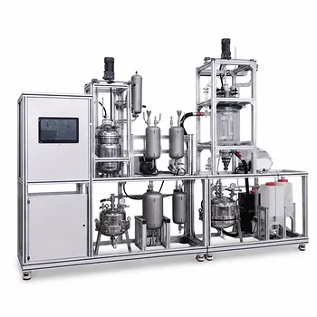
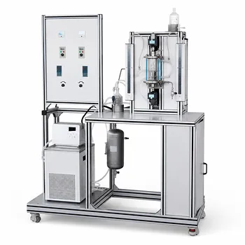
How Is The Rate Of Reaction Defined? Measure Kinetics With Batch, Cstr, And Pfr Pilot Plants

For a homogeneous liquid-phase reaction, the rate is the change in species amount per unit time and per unit volume of reacting fluid. For reactant (A), it is commonly written as (-r_A = -\frac{1}{V}\frac{dN_A}{dt}), with units such as (\mathrm{mol,L^{-1},s^{-1}}). If the liquid volume is constant, this becomes (-r_A = -\frac{dC_A}{dt}), where (C_A) is the concentration of (A). Educational pilot plants demonstrate this definition by measuring concentration changes with time in batch reactors or applying steady-state mass balances in CSTRs and PFRs.

The reaction rate is a local, intensive property determined by composition and operating conditions, not by reactor geometry. Pilot plants make the rate law measurable by combining controlled temperature, mixing, concentration, and residence time with online measurements such as conductivity, pH, pressure, absorbance, or flow.

What the Homogeneous Reaction Rate Means

Rate Based on Species Consumption

For a reactant (A), the negative sign ensures that the rate is positive while (A) is being consumed:

[ -r_A = -\frac{1}{V}\frac{dN_A}{dt} ]

Here, (N_A) is the amount of (A), (V) is the reacting-fluid volume, and (r_A) is the rate associated with species (A).

For a product (R), whose amount increases, the corresponding expression is:

[ r_R = \frac{1}{V}\frac{dN_R}{dt} ]

When a reaction has unequal stoichiometric coefficients, species rates should be related through the stoichiometry. A reaction rate normalized to the reaction progress avoids assigning different numerical rates to the same reaction simply because different species are measured.

Constant-Volume Liquid Systems

Most educational liquid-phase reactor experiments are designed to operate at approximately constant volume. Under that condition:

[ -r_A = -\frac{dC_A}{dt} ]

This form directly connects the measured concentration-time slope to the reaction rate.

The rate is an intensive quantity. Doubling the reactor volume does not change the rate per unit volume if temperature, composition, mixing, and other relevant conditions remain the same; it changes the total reaction rate and total material processed.

Rate Laws Are Algebraic Models

A kinetic rate law expresses the rate as an algebraic function of concentration and operating conditions:

[ -r_A = k(T)f(C_A,C_B,\ldots) ]

For example:

[ -r_A = kC_A ]

represents first-order dependence on (A), while:

[ -r_A = kC_A^2 ]

represents second-order dependence.

The rate law is not defined by whether the experiment uses a batch reactor, CSTR, or PFR. The reactor type determines how material balances convert the rate law into concentration profiles, conversion, or required volume.

Configuring a Pilot Plant for Kinetic Demonstrations

Batch Reactor for Concentration-Time Data

A jacketed, stirred batch reactor is the most direct configuration for teaching the definition of rate. Students charge known reactant concentrations, control the temperature, and record concentration or a concentration-related signal as the reaction proceeds.

The measured data provide (C_A(t)). Numerical differentiation or a fitted concentration model then gives:

[ -r_A = -\frac{dC_A}{dt} ]

A batch unit should include controlled agitation, temperature measurement and control, sampling access, and an online or at-line method for determining concentration.

CSTR for Steady-State Mass Balances

A continuous stirred-tank reactor operates at a controlled feed flow rate, feed composition, temperature, and liquid volume. Once steady state is reached, the reaction rate can be calculated from the material balance:

[ F_{A0}-F_A = (-r_A)V ]

For constant-density liquid systems, this can also be written in terms of concentration and volumetric flow rate:

[ Q(C_{A0}-C_A)=(-r_A)V ]

A CSTR therefore allows students to calculate the rate from inlet and outlet concentrations without differentiating noisy time-series data.

PFR for Rates Along the Reactor

A plug flow reactor provides concentration changes along reactor volume rather than primarily over elapsed batch time. Under steady-state conditions:

[ \frac{dF_A}{dV}=r_A ]

For a constant-density liquid and a reactant:

[ \frac{dC_A}{d\tau}=r_A ]

where (\tau) is the residence time. Multiple sampling points or inline sensors along the PFR make it possible to observe how concentration and local reaction rate vary through the reactor.

Instrumentation That Makes the Rate Visible

The sensor should measure a property that changes predictably with composition. Common choices include:

Conductivity: useful for ionic reactions, including the saponification of ethyl acetate.
pH: useful when hydrogen or hydroxide ions change significantly.
Spectrophotometry: useful for colored species or reactions with measurable absorbance.
Pressure or gas volume: useful when the reaction generates or consumes gas.
Flow and temperature sensors: necessary for residence-time calculations and temperature-dependent kinetic analysis.

The instrument signal must be calibrated against concentration. A conductivity value, for example, is not itself a reaction rate; it must be converted into concentration before the concentration change is interpreted kinetically.

Turning Measurements Into Kinetic Parameters

Demonstrating Reaction Order

Students can perform experiments at different initial concentrations and compare the measured rate with concentration. For a power-law model:

[ -r_A=kC_A^n ]

the exponent (n) is estimated from the concentration dependence of the rate.

For a second-order reaction, reciprocal concentration plots may be useful. For a first-order reaction in a batch reactor, a plot of (\ln C_A) against time should be approximately linear under ideal isothermal conditions.

Using a Pseudo-First-Order Experiment

If one reactant is present in large excess, its concentration may remain nearly constant. Consider:

[ -r_A=kC_AC_B ]

If (B) is in large excess, (kC_B) can be treated as an effective constant:

[ -r_A=k_{\mathrm{obs}}C_A ]

This configuration simplifies data analysis and allows students to estimate an observed rate constant from concentration-time data. The excess-reactant assumption should be checked experimentally rather than treated as automatically valid.

Estimating Temperature Dependence

The pilot plant can be operated at several controlled temperatures while keeping mixing, concentrations, and flow conditions consistent. The resulting rate constants can be analyzed using an Arrhenius relationship, commonly expressed as:

[ k(T)=k_0\exp\left(-\frac{E_a}{RT}\right) ]

A plot of (\ln k) against (1/T) can be used to estimate the activation energy (E_a) over a temperature range where the model is appropriate.

Demonstrating Saponification

The reaction between ethyl acetate and sodium hydroxide is a practical teaching example because conductivity can track the changing ionic composition:

[ \mathrm{CH_3COOC_2H_5 + OH^- \rightarrow CH_3COO^- + C_2H_5OH} ]

A batch reactor demonstrates concentration-time behavior. A CSTR demonstrates steady-state material balances, and a PFR demonstrates the relationship between conversion and residence time.

The measured conductivity must first be correlated with hydroxide or reactant concentration. Students can then compare candidate kinetic models and calculate rate constants under controlled conditions.

Understanding the Trade-offs

Reactor Type Does Not Change the Intrinsic Rate Law

The intrinsic rate law is associated with the reacting species and their local conditions. Reactor geometry affects mixing, residence-time distribution, heat transfer, and concentration variation, so it changes the observed reactor performance even though it does not fundamentally redefine the local homogeneous rate.

This distinction is central to reactor design: kinetics describe what happens locally, while reactor balances describe how that behavior accumulates throughout the equipment.

Differentiation Amplifies Experimental Noise

Calculating (-dC_A/dt) directly from measured batch data can be sensitive to sensor noise and sampling intervals. Smoothing, regression, or fitting an integrated kinetic model is often more reliable than taking raw point-to-point differences.

The analysis method should be reported because different smoothing or fitting choices can produce different apparent rate estimates.

Mixing and Temperature Can Distort Results

A batch reactor is only a useful kinetic reference when the liquid is adequately mixed and the temperature is sufficiently uniform. Poor mixing can create concentration gradients, while uncontrolled temperature changes can alter (k) during the experiment.

A CSTR also requires enough residence time to reach steady state. Using transient outlet data as though they represented steady-state behavior can produce an incorrect rate.

Series Reactions Require Careful Interpretation

For consecutive reactions such as:

[ A\rightarrow R\rightarrow S ]

the intermediate and final-product profiles depend on both rate constants and reactor conditions. If the second step is much faster than the first, (R) may remain at a low concentration and the first step can control the overall buildup of (S).

It is more accurate to describe this as a limiting kinetic regime than to state universally that the slowest step alone determines the complete reaction profile. Changing temperature or other conditions can alter the relative rate constants and shift which step is limiting.

Homogeneous and Heterogeneous Rates Use Different Bases

For homogeneous liquid systems, rates are generally reported per volume of reacting fluid, such as (\mathrm{mol,L^{-1},s^{-1}}). Heterogeneous catalytic systems are often normalized per catalyst mass, catalyst surface area, or another catalyst basis.

The normalization must match the physical system and be stated explicitly when comparing experiments.

Making the Right Choice for Your Goal

A pilot plant should be configured around the kinetic question being investigated:

If your primary focus is defining reaction rate: Use a temperature-controlled stirred batch reactor with calibrated concentration-sensitive instrumentation and calculate (-dC_A/dt) from concentration-time data.
If your primary focus is steady-state reactor design: Use a CSTR with controlled feed flow, reactor volume, inlet concentration, and outlet analysis so the rate follows from the steady-state mass balance.
If your primary focus is residence-time effects: Use a PFR with accurate flow measurement and concentration measurements at the outlet or along the reactor length.
If your primary focus is reaction order: Repeat experiments over several initial concentrations and fit the measured rates to competing algebraic rate laws.
If your primary focus is temperature dependence: Operate an isothermal batch or continuous unit at several temperatures and estimate (k) before applying an Arrhenius analysis.
If your primary focus is instrumentation and process monitoring: Select a reaction whose concentration is reliably correlated with conductivity, pH, absorbance, pressure, or gas volume, then validate the sensor calibration against independent samples.

A well-configured educational pilot plant connects controlled operating conditions, calibrated measurements, and material balances so that students can distinguish the reaction rate law from the reactor’s overall behavior.

Summary Table:

Kinetic objective	Recommended pilot plant	Key measurements or analysis
Define reaction rate	Temperature-controlled batch reactor	Concentration-time data and (-r_A=-dC_A/dt)
Apply steady-state balances	CSTR	Feed and outlet concentrations, flow rate, and reactor volume
Study residence-time effects	PFR	Flow rate, residence time, and concentration along the reactor
Determine reaction order	Batch or continuous reactor	Experiments at different concentrations and rate-law fitting
Estimate temperature dependence	Isothermal batch or continuous reactor	Rate constants at multiple temperatures and Arrhenius analysis
Demonstrate saponification	Batch, CSTR, or PFR	Conductivity calibrated against hydroxide concentration

Need a reliable way to teach reaction kinetics and reactor design? Contact LABPARK to discuss an educational or vocational unit operations pilot plant tailored to your goals. LABPARK provides configurable pilot plants for chemical engineering, bioprocess and biotech, and environmental and water treatment applications. Our systems help universities, research institutes, and enterprises demonstrate batch, CSTR, and PFR behavior, measure concentration with conductivity, pH, absorbance, pressure, or flow sensors, and connect experimental data with material balances, rate laws, reaction-order analysis, and Arrhenius modeling. Work with LABPARK to select the reactor configuration, instrumentation, controls, and teaching scope that fit your laboratory, research, or workforce-training needs.