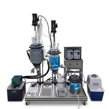
How Is Solubility Data Used To Select Solvents And Estimate Yields In Crystallization Unit Operations? A Guide

Solubility data isn't just a measurement—it's the decision‑making engine for every crystallization process.
Researchers and engineers use it to directly calculate the theoretical yield by comparing the mass of solute that remains dissolved at the dissolution temperature with the mass that stays in solution at the lower isolation temperature. This same data simultaneously guides solvent selection, ensuring the chosen solvent or solvent mixture delivers the highest recovery without sacrificing purity or process stability.

Crystallization design hinges on solubility data: a simple mass balance across the temperature drop predicts yield, while the shape of the solubility curve determines whether cooling, evaporation, or vacuum methods are viable. Selecting the optimal solvent requires balancing thermodynamic solubility thresholds with practical constraints like polymorph control, common‑ion effects, and throughput.

Estimating Crystallization Yield from Solubility Curves

The theoretical yield of a batch cooling crystallization is not an empirical guess—it flows directly from solubility values.

The Mass Balance Foundation

Yield is calculated by subtracting the mass of solute that remains dissolved at the final isolation temperature from the total mass dissolved at the initial hot dissolution temperature.
Because solubility is typically expressed as grams of solute per 100 grams of solvent (or as a molar fraction), you can convert these unit‑specific concentrations into absolute masses of dissolved solute.
The difference, divided by the starting mass, gives a theoretical yield percentage that purely thermodynamic considerations will allow.

In a properly designed pilot‑scale unit operation, this number becomes your upper‑bound recovery target.
Any real‑world losses—occlusion, clinging to vessel walls, or imperfect filtration—will reduce the actual harvested mass, but the theoretical yield remains the benchmark for process efficiency.

The van ’t Hoff Relationship as a Practical Tool

When solubility data is plotted using a linearized van ’t Hoff relationship (ln(solubility) versus 1/T), the resulting straight line makes yield prediction fast and visual.
If you know the solubility at your dissolution temperature and can read the solubility at your intended cooling endpoint, the mass balance reduces to a simple arithmetic operation using the known solvent mass.

This approach directly supports solvent screening.
Steep van ’t Hoff slopes indicate a high sensitivity to temperature change and thus large potential yields from cooling alone—making them prime candidates for an energy‑efficient process.
Shallow slopes warn that cooling alone will leave too much product behind, steering you toward evaporative or antisolvent crystallization instead.

Selecting the Optimal Solvent System

Solubility data determines not only how much product you recover, but also whether you recover the desired form and purity.

Matching Solvent to Temperature Dependence

The prime consideration in equipment selection is the shape of the solubility curve.
Compounds whose solubility decreases significantly as temperature drops are ideal for cooling crystallization—the most energy‑efficient and simplest to scale in a jacketed vessel.
When the solubility barely changes with temperature or even exhibits reverse solubility (more soluble at low temperature), cooling is useless; you must remove solvent via evaporative crystallization to force supersaturation.

For heat‑sensitive materials that fall in between, vacuum adiabatic cooling offers a middle path.
The vacuum simultaneously flashes off solvent and cools the solution, exploiting both effects.
Pilot‑scale teaching environments demonstrate these choices explicitly, showing students how a single solubility dataset dictates the entire hardware configuration.

Solvent Screening for Polymorph and Conformational Control

Solvent selection is a primary driver of polymorphic selectivity.
In a saturated solution, different solvents stabilize different molecular conformations. If the solvent environment favors a particular conformation, the crystal nuclei that form will overwhelmingly adopt the polymorph that matches that conformation.

A rational solvent‑screening protocol therefore requires not just high solubility, but solubility in a medium that preferentially populates the target conformer.
This decision is pivotal in pharmaceutical manufacturing, where the wrong polymorph can alter bioavailability or create patent disputes.
Pilot‑scale experiments often begin with thermodynamic predictions (such as COSMO‑RS) to shortlist solvents, then validate with small‑scale crystallizations before committing to a large batch.

The Role of the Solubility Product and Common Ion Effect

For ionic compounds, the solubility product (Ksp) replaces simple empirical solubility curves.
In a 1:1 electrolyte, solubility (s) equals the square root of Ksp, but non‑linear relationships (e.g., Ksp = 4s³ for a 2:1 salt) require more careful calculation.

This thermodynamic framework unlocks the common ion effect.
When you deliberately add an excess of a non‑target ion already present in your salt, the equilibrium shifts to reduce the solubility of the desired compound.
In a pilot plant, this means you can boost the recovery of a crystalline product without changing temperature or solvent—just by spiking a common ion salt.
Accurate Ksp data at operating temperatures makes these yield‑enhancement strategies predictable rather than trial‑and‑error.

Translating Solubility Data into Crystallization Method Choice

The same solubility measurements that forecast yield also dictate which unit operation hardware you should commission.

Cooling crystallization is the default when solubility drops sharply with temperature. A standard jacketed vessel with controlled cooling ramps is all that’s required.
Evaporative crystallization becomes necessary when the solubility curve is flat or inverse. You need a means to remove solvent—usually a heated vessel or a vacuum system—which raises energy costs.
Vacuum adiabatic cooling handles moderate temperature‑sensitivity profiles and protects heat‑labile products by combining flash evaporation with rapid cooling.

Understanding these boundaries at the pilot scale teaches an essential lesson: material properties drive process design, not the other way around.
If the solubility data says cooling won’t deliver the yield you need, no amount of vessel customization will fix it; you must switch to evaporation or antisolvent addition.

Leveraging Computational Predictions to Minimize Waste

Before committing solvent and solute to physical trial runs, computational thermodynamics now offers a fast screening stage.

Models like COSMO‑RS estimate the chemical potential difference between a compound in solution and in the solid state, predicting solubility limits across hundreds of solvent combinations.
In a pilot‑scale educational environment, students can run these predictions, select a handful of experimentally promising solvent mixtures, and then validate the results with 90% fewer wet‑lab trials.

This integration not only minimizes chemical waste but also teaches a critical skill: linking molecular‑scale thermodynamics directly to macroscopic unit operations like crystallization and extraction.
The theoretical yield maps generated computationally become the starting point for later empirical refinement on the pilot plant.

Understanding the Trade‑offs in Solvent Selection

A solvent that delivers a spectacular yield may still be the wrong choice if it compromises other crucial parameters.

Yield vs. Purity: A Delicate Balance

A solvent that dissolves your product exceptionally well at high temperature and almost not at all at low temperature gives you a huge theoretical yield.
But that same dissolution power often co‑dissolves impurities that will crash out alongside your product, ruining purity.

Alternatively, a very selective solvent may leave impurities in the mother liquor but also keep a significant fraction of your target compound dissolved—lowering yield.
Pilot‑scale work involves iterating over multiple solvent systems and crystallization conditions until you find the sweet spot where yield and purity meet your specification.

Throughput Constraints and Energy Efficiency

The volume of solvent required to achieve a given yield also determines reactor size and downstream processing time.
A system with moderate solubility at dissolution temperature demands more solvent mass per batch, increasing the cost of heating, cooling, and solvent recovery.
Even if the theoretical yield appears favorable on a percentage basis, the overall process economics can tip against it when you account for oversized equipment and high energy consumption.

Similarly, evaporative crystallization may raise yields for flat‑solubility compounds, but the energy needed to boil off large volumes of solvent can make the process uneconomical unless waste heat is available.
This is why solubility data must always be interpreted through an engineering‑economics lens, not just a thermodynamic one.

Making the Right Choice for Your Crystallization Goal

Your solubility dataset gives you the power to match process design to your exact priorities.

If your primary focus is maximizing recovery yield: Choose a solvent with a steep van ’t Hoff slope and, for ionic species, exploit the common ion effect to push equilibrium toward the solid phase.
If your primary focus is controlling polymorphic form: Screen solvents computationally first, then validate those that stabilize the target conformer, even if their raw yield is slightly lower.
If your primary focus is minimizing solvent use and waste: Use thermodynamic predictions like COSMO‑RS to shortlist high‑capacity solvents and design antisolvent mixtures that reduce total liquid volume.
If your primary focus is energy‑efficient operation: Stick with cooling crystallization for solutes with high temperature‑sensitivity; only pivot to evaporative or vacuum systems when the solubility curve demands it.

When you treat solubility data as the strategic roadmap rather than a mere physical constant, you transform a routine pilot‑plant run into a fully rationalized, scalable crystallization process.

Summary Table:

Crystallization Method	Solubility Curve Profile	Primary Equipment Needed
Cooling	Steep temperature dependence	Jacketed vessel with controlled cooling
Evaporative	Flat or inverse temperature dependence	Heated or vacuum vessel for solvent removal
Vacuum Adiabatic	Moderate sensitivity, heat-labile solute	Vacuum system with flash evaporation

Optimize Your Unit Operations Training with LABPARK

Bridging the gap between molecular thermodynamic data and industrial-scale execution requires hands-on experience. LABPARK provides state-of-the-art Educational and Vocational Unit Operations Pilot Plants in chemical engineering, bioprocess & biotech, and environmental & water treatment for universities, research institutes, and enterprises.

Ready to elevate your crystallization and process engineering curriculum? Contact us today to explore our customizable pilot plant solutions!