How Does Miscibility Affect Liquid-Liquid Extraction Pilot Plant Design? Key Calculation Workflows.

The miscibility of the carrier and solvent phases is the binary switch that dictates the entire mathematical framework for designing a liquid-liquid extraction pilot plant. For partially miscible systems, the internal flow rates of raffinate and extract change from stage to stage, so you must use ternary triangular diagrams and lever‑rule calculations to track phase compositions. For completely immiscible systems, the carrier (B) and solvent (S) flow rates remain constant throughout the cascade, allowing you to apply a simple straight operating line on X–Y coordinates (Yᵢ₊₁ = (B/S)Xᵢ + (Y₁ – (B/S)X_F)) and perform stage‑by‑stage calculations just as you would in binary distillation.

The critical insight: Miscibility is not a minor physical detail—it’s the fundamental parameter that decides whether you can simplify your design with constant flows and linear equations, or whether you must rely on the richer, but more complex, graphical world of ternary diagrams to capture changing internal phase flow rates.

The Two Calculation Paths Based on Phase Miscibility

The choice between a partially miscible and a completely immiscible model directly shapes the pilot plant’s design workflow, the data you need to measure, and the complexity of your stage‑to‑stage analysis.

For Partially Miscible Systems: Ternary Diagrams and Lever‑Rule

When the solvent and feed carrier dissolve in each other to a noticeable extent, the mass flow rates of the raffinate and extract phases are not constant. Every contact stage changes the composition, which in turn changes the amount of carrier that leaves in the extract or the amount of solvent that remains in the raffinate.

You must work with a ternary phase diagram (solute‑carrier‑solvent triangle) that shows the binodal curve and tie‑lines.
For each stage, you locate the equilibrium compositions via a tie‑line, then apply the lever‑arm rule to determine the relative amounts of the two coexisting phases.
Stage‑to‑stage mass balances are inherently graphical; you cannot reduce the process to a single straight operating line.
Pilot plants used for teaching or research often operate with partially miscible pairs (e.g., water‑acetone‑toluene) to demonstrate this procedure and to let students measure tie‑line data themselves.

For Completely Immiscible Systems: Straight Operating Lines and X–Y Coordinates

When the mutual solubility of the carrier and solvent is negligible, the entire design workflow simplifies dramatically. The flow rate of the carrier (B) remains unchanged throughout the cascade, and the solvent (S) flow rate is likewise constant.

You can plot the equilibrium relationship (solute concentration in extract vs. raffinate) on a rectangular X–Y diagram.
The operating line becomes a straight line with slope B/S: [ Y_{i+1} = \frac{B}{S} X_i + \left(Y_1 - \frac{B}{S} X_F\right) ]
You step off theoretical stages between the operating line and the equilibrium curve just as in a McCabe‑Thiele diagram.
This approach is central to many educational pilot plants because it provides a clean, quantitative link between the solvent‑to‑feed ratio (S/B), the extraction factor, and the required number of stages.

From Theory to Pilot Plant: A Practical Calculation Workflow

The lab‑scale pilot plant is where these two paths converge into a coherent design process. The workflow must accommodate which type of miscibility—partial or complete—governs the system.

Characterizing Phase Equilibrium at Pilot Scale

No reliable design can proceed without accurate liquid‑liquid equilibrium (LLE) data. The pilot plant itself is often used to measure the tie‑lines that build the ternary diagram or the distribution coefficient (K) for immiscible systems.

LLE solubility diagrams (temperature vs. mole fraction) reveal the boundaries of the two‑phase region and critical solution temperatures.
For systems with an upper critical solution temperature (UCST), operation must stay below the critical point; for those with a lower critical solution temperature (LCST), the column must be kept above the critical point.
Educational pilot plants deliberately vary temperature so students can observe how a single phase becomes two—directly tying the thermodynamic diagram to column behavior.

Selecting the Right Mathematical Framework

Once you know the degree of miscibility, you lock in your calculation method.

Significant mutual solubility (partial miscibility): Build or obtain a ternary diagram, and use the lever‑arm rule for stage‑to‑stage balances. This method accounts for the changing internal flow rates.
Negligible mutual solubility (complete immiscibility): Treat carrier and solvent flows as constant, construct an X–Y operating line, and count stages via the McCabe‑Thiele approach. This method also makes the extraction factor (Am = K·S/B) a powerful, single‑number performance indicator.

Incorporating Extraction Factor and Stage Efficiency

For immiscible systems, the extraction factor directly connects pilot plant operation to design economics. A higher Am (achieved by increasing the solvent flow rate relative to the feed carrier) reduces the number of theoretical stages—but demands more energy for downstream solvent recovery.

In a pilot plant, you can purposely vary the S/B ratio and measure the actual separation. The resulting data allows you to plot required stages versus Am, giving students a tangible grasp of the capital‑cost vs. operating‑cost trade‑off.
When partial miscibility prevails, the extraction factor concept is less straightforward because S and B are not invariant. However, you can still study the local trade‑offs by observing how the ternary tie‑lines shift with overall composition and temperature.

Understanding the Trade‑offs and Pitfalls

Miscibility assumptions carry real risks, and pilot plant design must guard against them.

Assuming complete immiscibility when partial miscibility exists leads to an underprediction of the required stages. The constant‑flow simplification neglects the fact that some solvent leaves with the raffinate and some carrier enters the extract, altering the effective L/G ratio in each stage.
Over‑complicating the workflow with ternary diagrams for systems that are, for all practical purposes, immiscible adds unnecessary complexity without a meaningful gain in accuracy. Time and effort are better spent on quick X–Y screening.
Extraction factor trade‑offs are only fully interpretable when S and B stay constant. If you adjust the solvent rate in a partially miscible system, you also shift the tie‑line contours, making a simple Am‑based optimization unreliable.
Temperature instability can unknowingly shift the system from a two‑phase region (where extraction works) to a single‑phase region (where it fails entirely), especially near a critical solution temperature. Pilot plants must maintain strict temperature control to stay within the desired miscibility regime.

How Physical Properties and Temperature Shape Miscibility and Design

The degree of miscibility is not a static label—it is heavily influenced by temperature and the solvent’s physical properties. A pilot plant design must account for these drivers.

The Role of Temperature in Defining Phase Boundaries

Temperature dictates whether two liquid phases can coexist. Binary LLE systems exhibit three typical behaviors, all directly relevant to pilot plant operation.

Systems with a UCST (e.g., phenol‑water) are fully miscible at high temperatures but split into two phases when cooled. The extraction column must be operated well below the critical point.
Systems with an LCST (e.g., water‑trimethylamine) are miscible at low temperatures and separate upon heating. In this case, you need to heat the system to stay in the two‑phase zone.
Systems with both UCST and LCST (e.g., water‑nicotine) only form two phases inside an intermediate temperature window. Outside that window, the mixture becomes a single phase and extraction stops.

Physical Properties That Determine Phase Separation

Even within the two‑phase region, the physical properties of the solvent and feed control how efficiently the phases disengage inside a pilot column.

A larger density difference, lower viscosity, and moderate surface tension accelerate droplet coalescence and settling.
Slow coalescence caused by high viscosity or a small density difference can lead to emulsions or phase entrainment, flooding the column at much lower throughput.
Pilot plant experiments that vary flow rate while monitoring the phase‑interface level directly teach these hydraulic limits, linking solvent choice to column hydrodynamics.

For solvent recovery, the design is driven by volatility: the solvent and feed components should have a high relative volatility and should not form azeotropes. If the solvent must be vaporized, a low latent heat of vaporization minimizes downstream utility cost. These solvent‑recovery requirements, combined with the phase‑separation properties and the miscibility regime, define the complete pilot plant design envelope.

Making the Right Choice for Your Goal

Your design and calculation workflow should be tailored to the specific purpose of the pilot plant and the real miscibility behavior of your system.

If your primary focus is rapid solvent screening and conceptual design: Assume complete immiscibility where possible, use constant‑flow X–Y diagrams, and leverage the extraction factor to quickly assess the trade‑off between stage count and solvent consumption.
If your primary focus is high‑fidelity process design for a system with measurable mutual solubility: Invest the time to construct the ternary phase diagram and apply lever‑rule stage calculations. This will yield the most accurate stage counts and flow‑rate profiles.
If your primary focus is education or fundamental research: Operate the pilot plant with both a partially miscible system (to teach ternary diagram methods) and an immiscible system (to teach McCabe‑Thiele‑style analysis and extraction factor concepts), allowing a side‑by‑side comparison of the two calculation philosophies.
If your primary focus is scaling up a known, temperature‑sensitive LLE system: Use the pilot plant to map the precise temperature boundaries where two phases exist, then select an operating point that guarantees robust phase separation while avoiding the single‑phase critical region.

The miscibility of your phases ultimately defines the mathematics you use, the pilot plant data you must collect, and the operational window you must obey. By aligning your design workflow with the real miscibility behaviour, you turn a fundamental thermodynamic property into the most powerful decision‑making tool in your extraction toolbox.

Summary Table:

Parameter	Partially Miscible Systems	Completely Immiscible Systems
Flow Rates	Variable stage-to-stage	Constant carrier ($B$) & solvent ($S$)
Calculation Method	Ternary diagrams & lever-arm rule	X-Y coordinates & straight operating line
Key Metric	Shifted tie-line contours	Extraction factor ($Am = K \cdot S/B$)
Primary Use Case	High-fidelity process modeling	Rapid screening & basic education

Optimize Your Chemical Engineering Lab with LABPARK

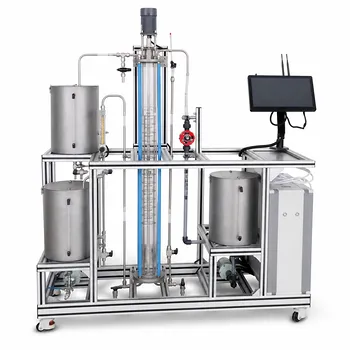
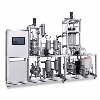
Are you looking to bridge the gap between liquid-liquid extraction theory and hands-on practice? LABPARK provides state-of-the-art Educational and Vocational Unit Operations Pilot Plants in chemical engineering, bioprocess & biotech, and environmental & water treatment.

Designed specifically for universities, research institutes, and enterprises, our pilot plants help students and researchers easily visualize phase behavior, master McCabe-Thiele and ternary diagram calculations, and scale up processes with confidence.

Ready to elevate your training and research capabilities? Contact LABPARK today to find the perfect pilot plant solution for your facility!