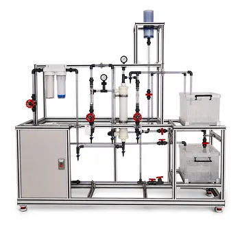
How Does Lu Decomposition Model Multi-Stage Systems? Optimize Your Pilot Plant Simulation

LU decomposition is the silent computational workhorse that turns complex pilot plant models into actionable, real-time insights. When chemical engineers model multi-stage unit operations—like a cascade of reactors or a distillation column—they are fundamentally building and solving large systems of linear algebraic equations derived from mass and energy balances. LU decomposition factorizes the coefficient matrix of these systems into lower and upper triangular forms, enabling a highly efficient two-step solution that drastically reduces computational load. This efficiency is what allows simulation and control software running on pilot plant hardware to keep pace with real-time process dynamics, making it an indispensable tool for bridging theory and physical reality.

Multi-stage pilot plant models boil down to solving Ax = b systems. LU decomposition is the most efficient direct method for this, turning a single, expensive matrix operation into a rapid, repeatable forward-and-back substitution that unlocks real-time simulation, on-the-fly optimization, and robust control system design—precisely the capabilities a pilot plant demands to validate and scale up chemical processes.

The Central Role of Linear Systems in Pilot Plant Modeling

Unit operations pilot plants serve as the critical bridge between bench-scale chemistry and full-scale industrial design. To fulfill that role, they must generate trustworthy data under controlled conditions, and mathematical models are the vehicle that transforms raw sensor readings into fundamental understanding.

Mass and Energy Balances as Linear Equations

At the heart of any chemical process model lies the conservation principle: what goes in must come out, or accumulate. For multi-stage systems—be they cascaded reactors, extraction batteries, or distillation trays—each stage generates a set of mass and energy balance equations.

When these balances are linearized around an operating point or expressed for steady-state conditions, they naturally form the familiar matrix equation Ax = b. The coefficient matrix A encodes the physical connectivity (flows, heat exchange) between stages, the vector x holds the unknown temperatures or concentrations, and b represents inlet conditions and external sources.

Multi-Stage Systems Amplify the Problem Size

A single stirred tank might yield a simple first-order differential equation. But a pilot plant with ten interconnected stages quickly generates a system of ten or more coupled equations. Solving these by brute-force substitution is impractical. The matrix A grows large and, although often sparse or banded, solving it efficiently becomes the critical bottleneck—especially when the model must run repeatedly for parameter sweeps, control tuning, or real-time simulation.

Why LU Decomposition is the Method of Choice

LU decomposition does not change the underlying physics; it changes how quickly you can extract the answer. The method factorizes A into a lower triangular matrix L and an upper triangular matrix U, with row pivoting to preserve numerical stability.

Factorization for Repeated Solutions

The beauty of LU decomposition is that the costly factorization step—the heavy lifting of Gaussian elimination—is done only once. After that, solving for different right-hand-side vectors b (different inlet conditions, process disturbances, or what-if scenarios) becomes a trivial two-step dance:

Forward substitution to solve Lz = b.
Back substitution to solve Ux = z.

For a pilot plant operator exploring multiple operating points or a control algorithm that must recalculate setpoints every second, this reusability is transformative. It slashes the computational effort from order n³ for each new solution to just order n², where n is the number of stages.

Computational Efficiency for Real-Time Applications

Pilot plants are increasingly used for process control validation and operator training simulators. The supplementary references highlight that the dynamic models behind these applications must run in sync with real physical time—a challenging requirement if the solver lags behind.

LU decomposition directly addresses this. Its lean arithmetic allows control software to quickly solve linearized plant models, enabling tasks like:

Real-time PID tuning: The controller can recalculate optimal parameters on the fly by repeatedly solving the linearized process model.
Model-based fault detection: Rapid comparison of predicted and actual sensor readings becomes feasible, helping diagnose fouling or equipment degradation.
Simulator responsiveness: Training simulators mirroring a multi-stage distillation or absorption pilot plant can deliver instantaneous feedback without artificial delays, creating a truly immersive learning experience.

Understanding the Trade-Offs

No numerical method is a silver bullet. LU decomposition’s effectiveness hinges on the nature of the problem, and acknowledging its limitations builds a more robust modeling practice.

Numerical Stability and Pivoting

The primary reference explicitly mentions “a version of Gaussian elimination with row pivoting.” Without pivoting, LU decomposition can fail or produce inaccurate results when the matrix A has very small diagonal elements compared to off-diagonal entries—a common scenario in stiff chemical systems with vastly different rate constants between stages.

Partial pivoting selects the largest available element as the pivot, dramatically improving stability. This step is computationally cheap and is the standard in any production-quality solver. Engineers must ensure their modeling tool uses pivoting, but once in place, LU remains a rock-solid choice for well-conditioned pilot plant matrices.

When Sparsity Changes the Game

Many multi-stage process matrices are banded or sparse, meaning most entries are zero. A dense LU factorization can introduce “fill-in,” creating non-zero entries where there were none, and thereby increasing memory and computation. For extremely large systems (e.g., a 1000-stage model), specialized sparse solvers may outperform a general-purpose LU algorithm.

However, in the context of a typical pilot plant with up to a few dozen stages, this trade-off is rarely a dealbreaker. The simplicity, availability, and predictable performance of LU decomposition make it the go-to tool, leaving the complexity of sparse methods for when the problem size genuinely demands it.

Making the Right Choice for Your Simulation Goal

The method you choose should mirror your pilot plant’s primary mission. LU decomposition is a leading solution, but its value is greatest when aligned with a specific objective.

If your primary focus is developing and tuning real-time control loops: Use LU decomposition. Its ability to rapidly re-solve the linearized model for changing setpoints and disturbances allows you to compute model-predictive control actions or adaptive PID gains within the control cycle time.
If your primary focus is high-fidelity operator training simulators: Implement LU decomposition as the core linear solver. It gives the simulator the speed needed to mimic real process dynamics without lag, preserving the training value and allowing “what-if” scenarios to be explored interactively.
If your primary focus is validating steady-state designs across hundreds of operating scenarios: Solve the base-case model once with LU, then simply reuse the factors with new right-hand sides. This turns a massive parametric study into a series of swift substitutions, shrinking weeks of calculation to hours.
If your primary focus is modeling extremely large or inherently sparse multi-stage networks: Start with LU decomposition, but profile your code. If fill-in becomes a measurable bottleneck, migrate to a sparse banded solver—while still appreciating that the same forward-elimination philosophy underlies most modern algorithms.

The mathematical models that give pilot plants their predictive power are built on linear systems, and LU decomposition is the tool that makes those systems solvable fast enough to bridge the gap from theory to real-time physical operation.

Summary Table:

Key Feature	LU Decomposition Advantage	Pilot Plant Impact
Reusability	One-time factorization, fast repeated solves	Enables real-time simulation & PID tuning
Efficiency	Reduces computational complexity from O(n³) to O(n²)	Handles complex multi-stage systems easily
Stability	Row pivoting prevents calculation failures	Ensures reliable models for stiff chemical processes

Bring Theory to Life with LABPARK Pilot Plants

Validating advanced mathematical models like LU decomposition requires precise, real-time physical data. LABPARK provides state-of-the-art Educational and Vocational Unit Operations Pilot Plants in chemical engineering, bioprocess & biotech, and environmental & water treatment for universities, research institutes, and enterprises. Our systems deliver the accuracy needed to align your digital simulations with physical reality.

Ready to upgrade your lab's capabilities? Contact our engineering experts today to find the perfect pilot plant solution!