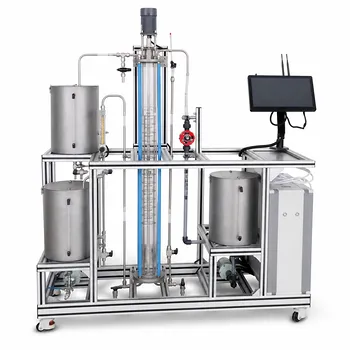
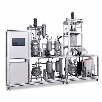
How Do Activity Coefficients Influence Distillation & Extraction Pilot Plant Design? Bridge Vle & Lle Theory.

Activity coefficients are the hidden architects of separation performance. In a chemical engineering pilot plant, they directly determine the phase equilibria that govern both distillation and liquid-liquid extraction. For distillation, the liquid-phase activity coefficient shapes the vapor-liquid equilibrium, fixing the relative volatility, the required number of trays, and the minimum reflux ratio. For extraction, the isoactivity condition ties solute distribution between two immiscible phases to the ratio of its activity coefficients, which drives solvent selection and stage count. When students calculate these coefficients using models like NRTL and then operate the pilot plant, they bridge molecular thermodynamics with the physical knobs of the process—solvent flow rates, feed locations, and energy inputs—transforming abstract theory into tangible design decisions.

Activity coefficients translate molecular non-ideality into the engineering variables that define a pilot plant’s size, operating policy, and separation efficiency. Mastering them is what turns a black-box unit operation into a predictable, optimizable system.

Why Activity Coefficients Sit at the Heart of Every Separation

A liquid mixture is rarely ideal. Activity coefficients quantify those deviations, and they appear inside the fundamental equilibrium equations that control distillation and extraction.

In a distillation column, the vapor‑liquid equilibrium is expressed through isofugacity. The liquid‑phase fugacity contains the activity coefficient ( \gamma_i ), which directly modifies the apparent vapor pressure of a component. This changes the relative volatility that governs the shape of the equilibrium curve.

In liquid‑liquid extraction, the equilibrium condition for a solute ( A ) between two liquid phases I and II is ( \gamma_A^{\text{I}} x_A^{\text{I}} = \gamma_A^{\text{II}} x_A^{\text{II}} ). The distribution coefficient is simply the ratio of the activity coefficients. If a student cannot predict that ratio, they cannot design the extraction cascade.

Influence on Distillation Pilot Plant Design and Operation

The Vapor‑Liquid Equilibrium Connection

Every tray or packing element in a distillation pilot column operates on the assumption of an equilibrium stage. That stage’s outlet compositions are fixed by the VLE relationship, in which ( y_i P = x_i \gamma_i P_i^{\text{sat}} ) (with appropriate fugacity corrections). The activity coefficient ( \gamma_i ) can amplify or suppress a component’s volatility. Strongly non‑ideal mixtures can form azeotropes, where ( \gamma_i ) makes relative volatility equal to one, stopping separation dead in its tracks.

For a student troubleshooting a pilot distillation run, a suddenly flat temperature profile often points to an azeotrope rooted in activity coefficient behavior. Understanding this keeps the plant operator from chasing an impossible purity.

Determining Column Height and Stage Requirements

Design methods like McCabe‑Thiele or rigorous simulation build the equilibrium curve directly from ( \gamma_i ). A larger departure from ideality frequently requires more theoretical stages for the same separation. In a pilot plant, that translates into a taller column—or more packed height—and higher capital footprint. Students learn that for polar‑nonpolar systems, the activity coefficients can be extreme enough to double the required number of stages compared to an ideal‑mixture assumption.

Operational Levers: Reflux Ratio and Energy Balance

Activity coefficients change with temperature, and not all components respond equally. In the ethanol/n‑octane system, a 30 °C increase cuts ethanol’s infinite‑dilution activity coefficient by nearly half while barely moving that of n‑octane. This differential temperature response directly alters relative volatility across the column’s thermal profile. The operator compensates by adjusting the reflux ratio and reboiler duty—decisions that directly impact the pilot plant’s energy balance. Students who see this effect firsthand never forget that thermodynamics is not a static constant but a dynamic driver of operating cost.

Influence on Liquid‑Liquid Extraction Pilot Plant Design and Operation

The Isoactivity Principle and Distribution Coefficients

In an extraction pilot plant, the solute partitions between the feed and solvent phases according to the isoactivity relationship. The distribution coefficient ( K = x_A^{\text{II}}/x_A^{\text{I}} = \gamma_A^{\text{I}}/\gamma_A^{\text{II}} ). The effectiveness of the entire solvent screening process hinges on predicting this ratio. A solvent that gives a favorable ( K ) in simulation only because of flawed activity coefficient predictions will disappoint in the real pilot runs. Students must learn that a solute’s love for one phase over the other is a direct expression of its activity coefficient contrast.

Solvent Selection and Stage Determination

With a model like NRTL or UNIQUAC, students can calculate ( \gamma_i ) for candidate solvents and estimate the required number of theoretical extraction stages. This activity‑coefficient‑based design is especially critical for polar or associating systems, where regular‑solution models fail. In a teaching pilot plant, comparing the predicted stage count with the observed separation provides a powerful lesson in model validation. A mismatch often reveals that VLE‑fitted parameters alone are insufficient; LLE data must be included in the fitting to capture the actual liquid‑liquid behavior.

Temperature Effects and Mass Transfer Optimization

Just as in distillation, temperature modifies activity coefficients in extraction. A small temperature swing can alter the distribution coefficient enough to shift the economically optimal solvent‑to‑feed ratio. In the pilot plant, students observe how cooling a mixer‑settler can boost extraction efficiency while simultaneously increasing viscosity and reducing mass transfer rates. This trade‑off lives wholly within the activity coefficient’s temperature dependence, teaching students to optimize a process, not just a formula.

Translating Theory into Practice: The Educational Bridge

From Molecular Thermodynamics to Unit Operations

The real power of a pilot plant curriculum lies in closing the loop. Students first calculate activity coefficients using NRTL with parameters from literature or simple group‑contribution methods. They then set the actual reflux ratio, feed tray, and solvent flow rate based on those calculations. When the plant runs, they compare the predicted tray temperatures, product purities, or raffinate concentrations with the measured values. This direct comparison forces a reckoning with the assumptions inside every thermodynamic model. The pilot plant becomes a physical truth‑test for the equations on the whiteboard.

Model Selection and Data Fitting

Polar and associating mixtures demand advanced local‑composition models like Wilson, NRTL, or UNIQUAC. For liquid‑liquid extraction in particular, using only VLE data to predict distribution coefficients is notoriously unreliable. A robust approach—taught in many pilot‑plant labs—is to fit binary VLE and LLE data simultaneously, then refine parameters with multicomponent LLE data. Students who perform this multi‑fitting exercise learn that activity coefficient models are not magic; they are correlations whose predictive power is limited by the quality of the underlying experiments.

Handling Non‑Ideality and Deviations

When a distillation run hits an unexpected azeotrope or an extraction reaches an early solubility limit, the culprit is usually an excess property. The excess Gibbs energy, from which activity coefficients are derived, encodes the non‑ideal behavior. By analyzing excess properties, students can pinpoint why the column is not hitting its target purity and adjust the feed stage or solvent‑to‑feed ratio accordingly. This habit of diagnosing a physical symptom with a thermodynamic root cause transforms a routine lab exercise into genuine process engineering.

Understanding the Trade‑offs

Activity coefficient models are essential, but they carry inherent limitations that any pilot‑plant education must address.

Model sensitivity to fitting data: An NRTL model fit only to VLE data can catastrophically mispredict liquid‑liquid equilibrium. The student must learn that the model’s value depends on the relevance and breadth of the data used.
Neglected vapor‑phase non‑ideality: Many activity coefficient models assume an ideal vapor phase or simple fugacity corrections. In high‑pressure or associating‑vapor systems, ignoring vapor‑phase non‑ideality introduces errors that the pilot‑plant measurements will expose.
Non‑equilibrium effects: Real packing and trays operate with finite mass transfer rates. The equilibrium‑stage model based on activity coefficients alone cannot capture tray efficiencies or axial mixing. Students must recognize when a efficiency correction is needed to reconcile the pilot‑plant data with the thermodynamic prediction.
Group‑contribution estimates vs. real mixtures: Tools like UNIFAC offer great predictive scope but can trade accuracy for generality. For a critical solvent screening task, relying solely on group contributions without any experimental tie‑point is a gamble that pilot‑plant time can’t afford.

How to Apply This to Your Educational Pilot Plant

Weave activity coefficient analysis into every design and debottlenecking exercise to build an instinct for non‑ideality.

If your primary goal is distillation design: Build VLE curves directly from ( \gamma_i ) models, test the impact of temperature‑dependent variations on relative volatility, and let students discover the minimum reflux and stage count for themselves.
If your primary goal is liquid‑liquid extraction: Use predicted ( \gamma_i ) ratios to screen solvents, then validate distribution coefficients with a single‑stage pilot experiment before scaling up to the full cascade.
If your goal is to teach robust thermodynamic modeling: Make students fit NRTL or UNIQUAC parameters from both VLE and LLE data, then force them to explain the observed pilot‑plant deviations in terms of the excess Gibbs energy.

When activity coefficients become the lens through which students view every temperature profile, composition profile, and solvent choice, the pilot plant stops being a piece of hardware and becomes a thermodynamic argument made visible—and that is the deepest education a unit operations lab can offer.

Summary Table:

Unit Operation	Key Thermodynamic Parameter	Direct Influence on Pilot Plant
Distillation	Vapor-Liquid Equilibrium ($y_i P = x_i \gamma_i P_i^{\text{sat}}$)	Determines relative volatility, minimum reflux ratio, and column height.
Liquid-Liquid Extraction	Isoactivity Condition ($K = \gamma_A^{\text{I}} / \gamma_A^{\text{II}}$)	Guides solvent selection, determines stage requirements, and optimizes partitioning.

Bring Molecular Thermodynamics to Life in Your Lab

Bridging complex thermodynamic theories with hands-on engineering is key to preparing the next generation of process engineers. LABPARK provides high-quality Educational and Vocational Unit Operations Pilot Plants in chemical engineering, bioprocess & biotech, and environmental & water treatment for universities, research institutes, and enterprises.

Ready to upgrade your laboratory curriculum and help your students master real-world process design? Contact us today to discuss your specific pilot plant requirements!