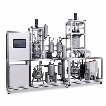
How Do Stepwise Stability Constants Guide Heavy Metal Recovery Pilot Plant Design? Maximize Capture Efficiency

Stepwise stability constants are the thermodynamic blueprint for controlling transition metal speciation in solution. By quantifying the stepwise association of each ligand molecule, they allow operators to calculate the exact equilibrium distribution of metal-ligand species (ML, ML₂, ML₃, …). In a heavy metal recovery pilot plant, this knowledge directly dictates the ligand dose required to shift the equilibrium overwhelmingly toward the fully saturated, most stable complex, preventing the formation of weakly coordinated intermediates that could decompose or escape capture during downstream separation.

The core takeaway: Stepwise stability constants enable deliberate control over which metal-ligand species predominate. The central operational rule is that to achieve robust heavy metal capture, operators must supply a stoichiometric excess of ligand—pushing the stepwise equilibria to the highest coordination number. This ensures the complex remains intact throughout filtration, precipitation, or solvent extraction, and it is the fundamental reason pilot plant design starts with a thermodynamic species-distribution calculation.

How Stepwise Constants Translate into Pilot Plant Control

A single formation constant (Kf) tells you only the stability of the final complex. Stepwise constants (K₁, K₂, … Kₙ) tell you how the metal gets there. This detailed speciation map is what makes pilot-scale separations predictable rather than empirical.

Mapping Free Ligand Concentration to Coordination State

Each stepwise equilibrium, such as (ML_{n-1} + L \rightleftharpoons ML_n), has its own constant. At a given free ligand concentration in solution, you can calculate the mole fraction of every species from (M^{n+}) to (ML_{\text{max}}).

This means the operator is not merely “adding ligand”—they are dialing in a specific free-ligand activity. A low ligand concentration may leave a significant fraction of metal as partially coordinated (ML) or (ML_2), which often carry residual charge, are more labile, and can break apart during pH shifts or temperature changes. Ramping up the free ligand drives the distribution toward the inert, highly coordinated end.

Selecting Ligand Dosage for Complete vs. Selective Complexation

If the goal is total recovery of all heavy metals, a large stoichiometric excess is chosen so that even the weakest last step (the step with the smallest Kₙ) is forced to completion. This is the strategy the primary reference highlights: excess ligand eliminates unstable intermediates and guarantees maximum complex stability under dynamic flow.

But stepwise constants also unlock selective separations. If two metals have markedly different K₁, K₂ values, a carefully controlled sub-stoichiometric ligand addition can fully complex one metal while leaving the other predominantly uncomplexed. That selectivity can be exploited in a cascade of reactors, where each stage targets a specific metal based on its unique stepwise profile.

Translating Thermodynamics into Pilot Plant Operation

A pilot plant runs under continuous-flow or batch-recycle conditions. Static equilibrium constants must be combined with kinetics and engineering constraints to produce reliable recovery.

Counteracting Dilution and Residence-Time Effects

In a continuous stirred-tank reactor (CSTR) or packed column, the metal and ligand are constantly being fed and removed. The residence time must be longer than the complexation reaction time. Because stepwise constants define the thermodynamic driving force for each step, they help engineers estimate whether a kinetic bottleneck exists. Metals with slow water-exchange rates may not reach the equilibrium distribution within the available residence time, even though the stability constants predict a favorable final state.

Adjusting for pH and Competing Equilibria

The free ligand concentration that matters for stepwise complexation is the unprotonated ligand activity. Many ligands (amines, carboxylates, EDTA) are weak bases. The apparent stepwise constants at a given pH drop dramatically if the ligand is protonated. Pilot plant design uses conditional stability constants—derived from the intrinsic stepwise constants and the ligand’s pKa values—to set the actual feed pH and total ligand concentration needed to maintain the target free-ligand level.

Understanding the Trade-offs and Common Pitfalls

Blindly applying “excess ligand” without considering the stepwise speciation can backfire. A few critical downsides must be managed.

The Economic and Fouling Cost of Over-Ligating

Ligand is often one of the most expensive consumables. The excess needed to force the last step (e.g., K₄ when K₃ is already large) may be 10–50 times the stoichiometric amount. That excess not only inflates operating costs but can also create a new waste problem: a high concentration of free ligand in the effluent may be toxic or interfere with downstream biological treatment.

Precipitate vs. Complex: Competing Pathways

The supplementary references highlight that heavy metals are often recovered by breaking complexes with sulfide precipitation. If you form an extremely stable high-coordination complex (high cumulative βₙ), the subsequent precipitation step requires a reagent that can outcompete that stability. For example, a fully coordinated EDTA complex of copper is far harder to break with sulfide than a partially coordinated ammine complex. Stepwise constants, paired with the solubility product (Ksp) of the target precipitate, allow you to choose a ligand that binds tightly enough for initial capture but releases the metal efficiently in the precipitation reactor. Over-stabilization is a common design mistake.

Ignoring the Weakest Link: The Last Stability Constant

The final stepwise constant, Kₙ, is often orders of magnitude smaller than K₁. Operators sometimes calculate the ligand dose based on the overall formation constant and assume complete complexation. In reality, if the free ligand concentration is insufficient, the MLₙ₋₁ species will persist. This intermediate may be exactly the species that passes through a nanofiltration membrane or adsorbs poorly onto an ion-exchange resin, causing early breakthrough and metal slip.

Making the Right Choice for Your Pilot Plant Goal

The design hinges on what you need the metal-ligand complex to do next. Use the stepwise stability constants to decode the speciation, and then match your operating conditions to the downstream unit operation.

If your primary focus is total metal capture before a membrane or IX column: Aim for the fully coordinated complex. Calculate the free ligand requirement from the smallest Kₙ, then add a safety margin. Continuously monitor free ligand in the reactor effluent, not just total metal, to confirm you are above the threshold where MLₙ dominates.
If your primary focus is selective recovery of one metal from a mixed stream: Map the species distributions for all metals at varying pL (free ligand concentration). Choose a dosage where the target metal is >99% complexed while competing metals remain predominantly free or weakly coordinated, enabling a separation stage ahead of the main precipitation step.
If your primary focus is precipitative recovery (e.g., sulfide or hydroxide): Do not maximize complex stability. Instead, use the stepwise constants in tandem with Ksp values to identify a ligand and coordination state that provides solution stability during transport but readily decomposes when the precipitating anion is added. The complex should be a temporary shuttle, not a thermodynamic sink.

Stepwise stability constants are not just academic data points—they are the control levers that let you dial in the exact metal speciation required for a robust, efficient, and selective heavy metal recovery pilot plant.

Summary Table:

Recovery Goal	Operational Strategy	Speciation Control Method
Total Metal Capture	Drive reaction to the highest coordination number	Add stoichiometric excess of ligand based on the smallest $K_n$
Selective Separation	Exploit differences in stepwise constants ($K_n$)	Control sub-stoichiometric ligand dosage to target specific metals
Precipitative Recovery	Enable easy ligand displacement for precipitation	Balance complex stability against precipitate solubility ($K_{sp}$)

Are you looking to optimize heavy metal recovery or scale up chemical separation processes? LABPARK provides high-quality Educational and Vocational Unit Operations Pilot Plants in chemical engineering, bioprocess & biotech, and environmental & water treatment. Specifically designed for universities, research institutes, and enterprises, our pilot plants enable precise control over complex chemical systems. Contact us today to find the perfect solution for your lab or facility!