How Do Impeller Type & Baffles Influence Nusselt Number? Optimize Pilot Plant Heat Transfer

The Nusselt number correlation in an agitated tank is not a fixed formula—it is a fingerprint of your specific mixing setup. The impeller type and the presence of baffles directly determine the constant C in the general correlation Nu = C * Re^a * Pr^b * (viscosity ratio)^c. In practice, a flat-blade turbine in a baffled tank at sufficient turbulence will give you C = 0.74, while the same turbine without baffles or at low speed may drop to C = 0.54. A propeller will give you C = 0.64, and a simple paddle may sit at a low 0.36. Baffles encourage the turbulent, high-shear flow regime that elevates the Nusselt number, while the impeller style sets the baseline mixing intensity reflected in C.

Core Insight: Baffles break the dominant tangential swirl, converting it into chaotic radial and axial motion that slashes the thermal boundary layer at the wall, giving a higher C in your Nusselt correlation. The impeller geometry defines the shear and pumping pattern, setting the starting value of C and the Reynolds number range where that enhancement kicks in. In a pilot plant, you must pick the correlation that exactly matches your baffle configuration, impeller type, and Reynolds number or you will misjudge the heat transfer area required.

How Baffles Transform Heat Transfer Correlations

In an unbaffled cylindrical tank, the impeller primarily spins the fluid in a tangential circle. This creates a central vortex, but it produces very little relative velocity between the fluid layers and the vessel wall. The result is a thick thermal boundary layer and a poor heat transfer coefficient. When you install baffles—typically four vertical flat plates equally spaced around the wall—they abruptly redirect that swirl into a powerful radial and axial secondary circulation. The fluid is thrust against the wall, scraped along the baffle edges, and constantly renewed at the heat transfer surface. That sharp increase in wall shear directly translates to a higher Nusselt number.

Quantifying the Jump in the Correlation Constant

The primary reference gives a clear example with flat-blade disk turbines. Below a Reynolds number of 400, the correlation Nu = 0.54 * Re^0.67 * Pr^0.33 * (viscosity ratio)^0.14 applies whether baffles are present or not—the flow is relatively gentle in either case. But once Re > 400 inside a baffled vessel, the constant leaps to 0.74. That 37% increase in C reflects the transition to a fully turbulent, baffle-induced mixing regime. In contrast, the same turbine in an unbaffled tank simply spins the fluid faster without proportionally boosting wall heat transfer, so the higher constant should not be used. For a pilot plant, this means that a cooling jacket sized using the unbaffled correlation will be dangerously undersized if you later operate with baffles in turbulent flow.

Why the Exponents Often Stay the Same

You will notice that for most impeller-wall heat transfer, the Reynolds exponent remains 0.67, and the Prandtl number exponent stays at 0.33. These exponents capture the fundamental physics of convective heat transfer in turbulent, non‑boiling liquids. The configuration change (baffles vs. no baffles) largely alters the intensity of that turbulence, not its nature. Therefore, the correction is packed almost entirely into the leading constant C. This is why simply reading a general “agitated vessel Nusselt correlation” from a textbook without checking the baffle status can lead to a 40% or larger error in the predicted heat transfer coefficient.

Impeller Geometry: The Constant Factor in Heat Transfer

Even with baffles, the impeller shape determines the starting point of the Nusselt correlation. A high‑shear radial turbine, an axial‑pumping propeller, and a low‑shear paddle each create a different local flow pattern around the blades, which in turn determines how effectively the fluid is churned against the wall.

Flat‑Blade Paddles versus Disk Turbines

For a simple two‑ or four‑blade flat‑blade agitator (often called a paddle), the correlation is Nu = 0.36 * Re^0.67 * Pr^0.33 * (viscosity ratio)^0.14 for Re < 4000. The constant is low because these impellers cause gentle sweeping motion with limited radial discharge. A flat‑blade disk turbine, with its blades placed on a central disk, forces a much stronger radial flow and shear. This directly lifts the constant to 0.54 (for Re < 400) and, as we saw, to 0.74 in a baffled tank at Re > 400. In a pilot plant, if you upgrade from a paddle to a disk turbine while keeping the motor speed constant, you will see the wall heat transfer coefficient jump by about 50% purely because of the increased turbulence.

Axial Propellers and Internal Coils

A three‑blade marine propeller operating at Re > 5000 yields Nu = 0.64 * Re^0.67 * Pr^0.33 * (viscosity ratio)^0.14. The constant sits between the low‑Re disk turbine and the baffled high‑Re turbine—a reflection of the strong axial flow that directs fluid along the wall rather than violently against it. When heat transfer is directed to internal helical coils, a separate correlation applies. For a flat‑blade turbine on a coil, Nu = 1.10 * Re^0.62 * Pr^0.33 * (viscosity ratio)^0.14 for 2000 < Re < 700,000. Note the Reynolds exponent shifts to 0.62 because the coil geometry changes the flow resistance at the heat transfer surface. Therefore, in a pilot plant, never apply a wall‑jacket correlation to an internal coil system.

Understanding the Trade-offs

Choosing an impeller and baffle configuration for optimal heat transfer is never a one‑sided decision. Every enhancement brings a real cost in energy consumption, mechanical complexity, or product quality.

Higher Heat Transfer Comes at a Power Cost

Baffles and high‑shear impellers like disk turbines require significantly more power. The power number of a disk turbine in a baffled tank can be five to ten times higher than that of a propeller or paddle in an unbaffled one. For a pilot plant, that means a larger motor, more cooling water, and often a stronger shaft. You must weigh the reduced heat transfer area (due to a higher C) against the increased electrical load. Frequently, the economic optimum lies somewhere between the extremes.

Shear Sensitivity and Dead Zones

The same strong turbulence that boosts the Nusselt number may damage shear‑sensitive cells, polymers, or crystals. In such cases, a low‑shear axial impeller with baffles is often a better compromise—it maintains uniform temperature without destroying the product. However, even with baffles, a single impeller can still leave stagnant zones below or above it, which can cause the real mixing time to diverge from the model and create hot spots. Adding a second impeller, as the supplementary references note, drives the residence‑time distribution toward near‑ideal behavior, ensuring that the Nusselt correlation’s assumption of a perfectly mixed fluid is actually met.

Scale‑Up Limitations of Pilot Plant Correlations

All the given correlations assume geometric similarity (standard baffle width, impeller diameter, liquid height). In a pilot plant, you may deliberately vary these to suit a particular experiment. If your baffle width is half the standard, or your impeller is positioned off‑center, the derived Nusselt number can deviate by ±20% or more. Always verify your configuration against the specifics of the correlation’s development, and when in doubt, measure the heat transfer coefficient directly in the pilot run.

Making the Right Choice for Your Pilot Plant Experiment

Your decision should be driven by what you are ultimately trying to model or demonstrate. Select your impeller and baffle combination to match the physics you care about.

If your primary focus is scaling up a heating/cooling step for a future production reactor: Use a fully baffled vessel with a flat‑blade disk turbine to achieve the highest possible C (0.74 at Re > 400). Then validate the calculated jacket area with one or two pilot‑scale heat‑up tests, because volumetric scale‑up amplifies any error in C.
If your primary focus is mixing a shear‑sensitive fluid with reliable heat removal: Choose a low‑shear axial impeller (e.g., a marine propeller) with baffles to get a moderate constant (around 0.64) while preserving the product. Configure with two impellers if vessel height is more than one diameter to prevent dead zones.
If your primary focus is teaching students the direct effect of baffles: Run the same impeller at the same speed with and without baffles. Use the Re < 400 correlation (C=0.54) as a baseline for the unbaffled case, then demonstrate that the jacketed temperature drop is far larger with baffles, even though the correlation’s constant technically stays at 0.54 until Re > 400. This highlights that the correlation valid ranges are just as important as the numbers.
If your primary focus is heat transfer to an internal coil: Use the dedicated coil correlation (Nu = 1.10 * Re^0.62 …) with a flat‑blade turbine. Do not attempt to adapt a wall‑jacket correlation, because the flow field around the coil differs fundamentally from the wall boundary layer.

The right correlation in your pilot plant puts the physical reality of baffles and impeller type into a mathematical form you can trust. Clarity on these driving forces avoids the most common scaling mistakes and ensures your experimental data translates faithfully to the next production scale.

Summary Table:

Impeller Type	Baffle Configuration	Reynolds Number (Re)	Constant (C)	Flow Characteristics
Flat-Blade Disk Turbine	Baffled	Re > 400	0.74	High-shear, turbulent radial flow; maximum heat transfer
Flat-Blade Disk Turbine	Unbaffled	Re < 400	0.54	Gentle, transitional flow; lower thermal renewal at wall
Marine Propeller	Baffled	Re > 5000	0.64	Strong axial flow; moderate shear for sensitive media
Flat-Blade Paddle	Baffled/Unbaffled	Re < 4000	0.36	Low shear; gentle sweeping with minimal radial discharge
Flat-Blade Turbine (Coil)	Internal Helical Coil	2,000 - 700,000	1.10	Flow modified by coil geometry (Re exponent shifts to 0.62)

Optimize Your Scaling and Teaching with LABPARK Pilot Plants

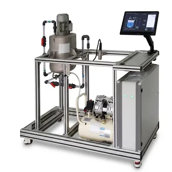
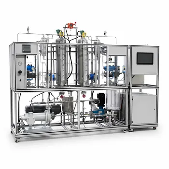
Need to validate heat transfer correlations or demonstrate chemical engineering principles in real-world scenarios? LABPARK provides premium Educational and Vocational Unit Operations Pilot Plants in chemical engineering, bioprocess & biotech, and environmental & water treatment.

Designed specifically for universities, research institutes, and enterprises, our systems allow hands-on configuration of impellers, baffles, and coils to match your exact modeling needs.

Ready to elevate your lab's capabilities? Contact LABPARK today to discuss our custom pilot plant solutions!