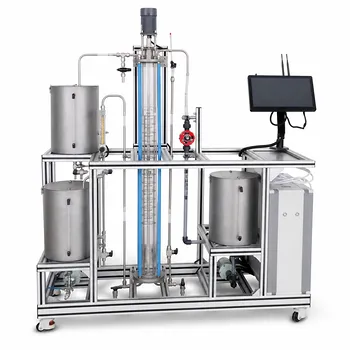
Educational distillation column pilot plants make material-balance and degree-of-freedom analysis tangible by connecting equations to measured process streams. Students define system boundaries around the column and reboiler, identify feed, distillate, bottoms, reflux, and internal vapor-liquid streams, and use measured flow rates and compositions to formulate overall and component balances. They can then determine whether the model is solvable before calculating component recoveries, product distributions, or separation performance.

A pilot plant turns degree-of-freedom analysis from an abstract counting exercise into a practical test of whether a real process has enough independent measurements and equations to describe its operation.

How the Pilot Plant Defines the Problem

Establishing the System Boundary

A continuous distillation column is an open, steady-state system: material enters continuously, products leave continuously, and the inventories inside the chosen boundary remain approximately constant.

Students may draw a boundary around the entire column and reboiler, or analyze smaller subsystems such as the condenser, reboiler, or a selected column section. The boundary determines which streams are treated as external inputs and outputs and which are internal process streams.

Separating External and Internal Streams

For an overall column-and-reboiler boundary, the principal external streams are usually the feed, overhead distillate, and bottoms product. Reflux and boil-up are internal to that boundary, so they do not appear in the overall material balance.

This distinction teaches an important modeling principle: internal streams influence separation behavior, but they cancel from an overall balance when they do not cross the selected boundary.

Using a Binary Mixture

A binary system such as ethanol and water provides a manageable example. The process can be described using total flow rates and the composition of one independent component, because the two component fractions in each stream must sum to one.

For a nonreactive steady-state system, students can write:

[ F = D + B ]

for the overall balance, and:

[ Fz_i = Dx_i + By_i ]

for component (i), where (F), (D), and (B) are feed, distillate, and bottoms flow rates, while (z_i), (x_i), and (y_i) represent the corresponding component fractions.

How Material Balances Are Built

Counting Independent Balances

The overall balance and component balances are related. For a binary nonreactive mixture, the two component balances imply the overall balance when stream compositions are properly normalized, so students must avoid counting dependent equations as independent.

More generally, the maximum number of independent component material balances equals the number of independent chemical species balances after accounting for composition-sum constraints and any reactions.

Applying Measured Operating Data

Pilot plants provide data such as feed flow rate, feed composition, distillate composition, bottoms flow rate, reflux flow rate, temperatures, pressures, and reboiler or condenser duties.

Students use these measurements to substitute known values into the balance equations. The remaining unknown flow rates or compositions can then be calculated using linear algebra or direct solution of the balance equations.

Calculating Component Recovery

Once stream flow rates and compositions are known, students can determine how the target component is distributed between products. For example, recovery of component (i) in the distillate can be expressed as:

[ \text{Recovery}_{i,D}

\frac{Dx_i}{Fz_i} ]

This connects conservation laws to a meaningful process metric: how effectively the column directs a desired component into a specified product stream.

Evaluating Material-Balance Closure

Measured data rarely satisfy the balances exactly because of instrument uncertainty, sampling error, leaks, holdup changes, or unmeasured streams. Students therefore compare total measured input with total measured output and calculate a material-balance closure or discrepancy.

A significant discrepancy may indicate sensor calibration drift, incorrect composition measurements, unsteady operation, reboiler or condenser problems, or an unmetered loss. This makes the balance a diagnostic tool rather than merely an algebraic exercise.

How Degree-of-Freedom Analysis Guides the Work

Identifying Unknown Variables

Students first list every unknown crossing the chosen system boundary. These may include stream flow rates, component fractions, reflux rates, product compositions, temperatures, or heat duties.

The list must be explicit. A variable that is not measured, specified, or otherwise known remains an unknown even if it seems operationally obvious.

Counting Independent Equations

The next step is to count independent relationships available to solve those unknowns. Depending on the scope of the model, these may include:

Overall and component material balances
Composition summations
Reflux or split specifications
Vapor-liquid equilibrium relations
Energy balances
Enthalpy or physical-property relationships
Measured operating conditions

The equations must be independent. Adding a redundant equation does not increase the information available to solve the model.

Interpreting the Degree of Freedom

The degree of freedom is calculated as:

[ N_D = N_U - N_E ]

where (N_U) is the number of unknown variables and (N_E) is the number of independent equations.

(N_D = 0): The model is exactly specified and can have a unique solution.
(N_D > 0): The model is underspecified and requires additional measurements or process specifications.
(N_D < 0): The model is overspecified, meaning measurements or equations may be redundant or inconsistent.

This analysis tells students whether it is appropriate to proceed with calculations and helps them identify which missing measurement would provide the most useful additional information.

Linking DOF Analysis to Instrumentation

A pilot plant demonstrates that solvability depends partly on instrumentation. If students know feed flow but lack a bottoms flow or product composition, the balance system may remain underspecified.

Conversely, collecting many measurements does not automatically improve the model. Measurements that repeat the same information can create an overspecified system without resolving the underlying uncertainty.

What Students Learn From Reflux and Internal Flows

Understanding Why Reflux Matters

Although reflux may cancel from an overall column balance, it strongly affects the internal vapor-liquid traffic and the separation achieved by the column.

The reflux ratio is commonly defined as:

[ R = \frac{L}{D} ]

where (L) is the condensed liquid returned to the column and (D) is the distillate product flow rate. Changing this ratio allows students to observe how internal liquid recycling affects product composition and recovery.

Connecting Balances to Separation Theory

By varying reflux and measuring distillate and bottoms compositions, students can compare experimental results with vapor-liquid equilibrium models and methods such as McCabe-Thiele analysis.

Temperature profiles along trays or packing provide additional evidence of changing phase compositions. These observations connect component balances with the physical mechanism of distillation: repeated vapor-liquid contact and preferential transfer of more volatile components.

Extending the Model to Energy Balances

A material-balance model may be sufficient for calculating flow distributions, but a broader pilot-plant analysis can include the reboiler and condenser energy duties.

Students can relate measured heat input, condensation duty, sensible heating, latent heat, and feed preheating to overall energy consumption. In multi-column systems, they can also evaluate energy recovery when a hot bottoms stream preheats a colder feed.

Understanding the Trade-offs

Measurement Realism Versus Model Simplicity

A simplified binary steady-state model is easier to solve and interpret, but it omits effects present in real operation. A more complete model may include energy balances, multiple components, pressure variation, phase equilibrium, tray efficiency, and changing holdup.

The educational value lies in comparing these model levels. Students see which assumptions make the equations manageable and which operating details must be restored for higher-fidelity predictions.

Steady-State Assumptions Versus Actual Operation

The steady-state assumption requires flows, compositions, temperatures, and inventories to be sufficiently stable. Startup, shutdown, reflux changes, and batch operation violate this assumption and require transient balances.

Batch distillation is particularly useful for showing that distillate composition can change with time at a constant reflux ratio. It illustrates why a balance that is valid for a continuous steady-state column cannot be applied unchanged to a dynamic process.

More Measurements Versus Better Measurements

Additional sensors can reduce uncertainty, but they also introduce calibration requirements, data reconciliation issues, and the possibility of conflicting measurements.

Students should distinguish between an underspecified model, which lacks information, and an overspecified model, which has more reported information than can be made mutually consistent. Material-balance closure helps evaluate the quality of the measurement set.

Overall Balances Versus Detailed Column Models

An overall balance can determine product flow distributions without describing what happens on each tray or packing section. It cannot, by itself, determine stage efficiency, internal composition profiles, or the number of theoretical stages.

Those questions require additional equilibrium, energy, and transport relationships. The pilot plant helps students understand that the choice of system boundary controls both the usefulness and the limitations of the resulting model.

Making the Right Choice for Your Goal

A practical workflow is to define the boundary, list known and unknown variables, count only independent equations, solve the balance model, and then compare predictions with measured data.

If your primary focus is material accounting: Use feed, distillate, bottoms, and composition measurements to perform overall and component balances and calculate product recoveries.
If your primary focus is model solvability: Complete a degree-of-freedom analysis before solving equations, then identify the missing measurement or specification when (N_D > 0).
If your primary focus is measurement validation: Calculate material-balance closure and investigate discrepancies through calibration checks, sampling review, and inspection for unmetered losses.
If your primary focus is separation performance: Vary reflux ratio and use product compositions, temperature profiles, and flow distributions to compare pilot-plant behavior with equilibrium and stage-based theory.
If your primary focus is energy efficiency: Expand the boundary to include reboiler, condenser, preheater, or heat-exchanger duties and perform coupled material and energy balances.

Educational distillation pilot plants teach students to treat balances and degrees of freedom as practical tools for building, testing, and improving process models.

Summary Table:

Focus Area	What Students Learn	Key Outputs
System boundaries	Distinguish external streams from internal reflux and boil-up flows	Correct process model
Material balances	Apply overall and component balances to binary mixtures	Flow rates and compositions
Degree-of-freedom analysis	Compare unknown variables with independent equations	Solvable model and data requirements
Measurement validation	Use closure calculations to identify errors, leaks, or missing data	Improved data reliability
Separation performance	Relate reflux, compositions, and temperature profiles to separation theory	Recovery and product-quality analysis
Energy analysis	Extend the model to reboiler, condenser, and heat-exchanger duties	Energy-use insights

Equip your students, researchers, or process-development team with hands-on experience using real chemical engineering data. Contact LABPARK to discuss Educational and Vocational Unit Operations Pilot Plants for distillation and other chemical engineering applications. LABPARK also provides pilot plants for bioprocess and biotechnology, plus environmental and water treatment. Our systems help universities, research institutes, and enterprises teach material balances, validate measurements, evaluate separation performance, and connect process theory with industrial practice.