Pay close attention to your data density. Students can dramatically optimize the accuracy of ASTM-to-TBP conversions in pilot plant operations by significantly increasing the number of input ASTM D86 data points, particularly in temperature regions where the distillation curve shows sharp deviations or steep slopes. More data points force the conversion algorithm to produce finer, more precise linear approximations for the ASTM and API curves, directly preventing interpolation errors and ensuring the generation of highly accurate pseudocomponents.
Accurate TBP curves are the bedrock of pilot plant modeling—they determine your pseudocomponent definitions, physical property estimates, and ultimately the fidelity of your mass balances and column performance predictions. The single most impactful action a student can take is to strategically add ASTM data points in the steep-slope regions, because that is where the piecewise-linear conversion is most vulnerable to large interpolation errors.
Why ASTM-to-TBP Conversion Accuracy Matters in Pilot Plants
Before diving into the optimization technique, it is essential to understand what rests on the outcome. In unit operations pilot plants, you rarely analyze thousands of individual species. Instead, you rely on laboratory standards like ASTM D86 and then apply mathematical conversions to create a True Boiling Point (TBP) curve.
The Pseudocomponent Connection
The TBP curve is not the endpoint. It is used to define discrete boiling fractions, or pseudocomponents. Each pseudocomponent carries a set of estimated physical properties—molecular weight, critical temperature, critical pressure, and acentric factor—that feed directly into your process simulator.
From Laboratory Data to Column Performance
Without an accurate TBP database, every subsequent calculation degrades. Shortcut methods like Fenske-Underwood-Gilliland and rigorous MESH equation solvers both rely on these property packages. When you compare simulation outputs with real-time pilot plant data (temperatures, flow rates), the quality of your TBP conversion determines whether the discrepancy is a meaningful insight or a self-inflicted artifact.
The Core Optimization Strategy: Denser Data in Steep Regions
The primary reference identifies a single, high-leverage action: increase the number of input ASTM data points in temperature regions showing sharp deviations or steep slopes.
How the Conversion Algorithm Treats Your Data
The typical API method-based conversion works by constructing piecewise-linear relationships between your ASTM data points and the corresponding curves. Each pair of consecutive data points defines a linear segment. If those points are far apart on a steep section of the curve, linear interpolation can significantly misrepresent the true boiling behavior.
Why Steep Slopes Multiply Interpolation Errors
On a flat section of the curve, spreading points further apart introduces minimal error because the slope is nearly constant. However, on a steep slope—common in the front end (gasoline range) or near the initial boiling point—a single linear segment replaces a rapidly changing temperature profile. This distortion cascades into inaccurate pseudocomponent cut points and incorrect property assignments.
Practical Steps for Students During the Lab
While collecting ASTM D86 data, observe the temperature–volume plotting in real time. The moment you notice the slope increasing or a sudden inflection, reduce the cumulative volume increment between recorded readings. For example, instead of recording at every 10 mL, switch to every 2–5 mL through the steep region. The goal is to feed those extra coordinates directly into the conversion algorithm, forcing it to use more linear segments and thus sharply reducing interpolation error.
The Ripple Effect: How Better TBP Curves Improve Pilot Plant Learning
Optimizing the TBP conversion is not an isolated academic exercise. It directly strengthens the educational bridge between simulation and reality.
Tighter Pseudocomponent Definition for Rigorous Models
With more precise TBP data, the pseudocomponents you define will carry more accurate critical properties. This makes your rigorous column models (Naphtali-Sandholm or inside-out methods) much more trustworthy when you later compare calculated tray temperatures and product compositions against physical sensor readings.
Validating Efficiency and Separation Boundaries
When you analyze tray efficiency—whether by the O’Connell correlation or the more detailed two-film method—the fluid properties derived from your pseudocomponents must be correct. Similarly, ternary residue curve maps and phase equilibrium diagrams rely on the same property database. A small error in the TBP curve can shift a feed composition across a distillation boundary, leading to completely wrong predictions about product recoverable as distillate versus residue.
Understanding the Trade-offs and Limitations
While increasing data point density is powerful, students must also recognize the method’s boundaries.
The Conversion Itself Is an Approximation
The API method, even when fed dense data, is an empirical correlation. It cannot capture every nuance of a highly complex mixture. Expect that the resulting TBP curve is a smoother, idealized representation—not a perfect reflection of a true 15/5 theoretical plate distillation.
Practical Constraints in the Laboratory
Collecting many extra data points takes time and may challenge sample volume constraints. There is a point of diminishing returns where adding more points does not meaningfully improve the linear segment accuracy. Students should focus the extra effort on regions where the ASTM slope visibly changes, rather than uniformly oversampling the entire curve.
The Lumped Nature of Pseudocomponents Remains
Even a perfect TBP conversion still divides the mixture into an arbitrary number of lumps. The choice of how many pseudocomponents you define will still influence column simulation accuracy. The strategy here ensures that those lumps are carved at the right temperatures, but the lumping philosophy itself is a separate design decision.
Making the Right Choice for Your Pilot Plant Goal
Apply the increased data density strategy where it matters most for your specific analysis objective.
- If your primary focus is rigorous simulation of product splits: Concentrate extra ASTM data points in the temperature range spanning your Light Key and Heavy Key components. This ensures that the pseudocomponent distribution in the fractionation zone is accurately represented, so the column’s separation power is calculated on a realistic feed.
- If your primary focus is energy balance and column diameter sizing: Add supplementary points across the entire boiling range, with extra focus on the heavy residue end. Errors in the high-boiling pseudocomponents can distort reboiler duty, column temperature profile, and vapor load estimates far more than similar errors in the light ends.
- If your primary focus is educational validation of tray efficiency: Use the densest dataset you can practically collect to generate TBP curves for each feed batch. Then apply the Murphree efficiency calculations with confidence that the theoretical stage requirements you derive from the TBP are not biased by interpolation errors, allowing you to isolate real hydrodynamic effects.
Master the simple discipline of strategic data input, and your ASTM-to-TBP conversion becomes a trusted foundation—not a hidden source of error—for every simulation, calculation, and physical pilot plant insight that follows.
Summary Table:
| Distillation Region | Slope Profile | Recommended Data Density | Impact on Pilot Plant Simulation |
|---|---|---|---|
| Front End / IBP | Steep / Rapid change | High (Every 2–5 mL) | Prevents interpolation errors; defines accurate light key components. |
| Mid-Boiling Range | Flat / Steady | Standard (Every 10 mL) | Saves lab time without sacrificing property estimation quality. |
| Heavy Residue End | Steep / Tail | High (Extra points) | Ensures correct reboiler duty and column vapor load sizing. |
Elevate Your Chemical Engineering Lab with LABPARK
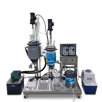
Bridge the gap between distillation theory and real-world application. LABPARK offers premium Educational and Vocational Unit Operations Pilot Plants in chemical engineering, bioprocess & biotech, and environmental & water treatment. Tailored for universities, research institutes, and enterprises, our pilot plants empower students to master complex process modeling with precision.
Ready to upgrade your lab's training capabilities? Contact us today to request a quote!
Related Products
- Multi-Modal Distillation Unit Operations Training Pilot Plant
- Multi-Functional Special Distillation Educational Pilot Plant
- Continuous Batch Extractive Distillation Educational Pilot Plant
- Green Anhydrous Ethanol Purification Extractive Distillation Unit Operations Training Pilot Plant
- Continuous Sieve-Plate Distillation Pilot Plant for Unit Operations Laboratory Education
People Also Ask
- How can energy balance equations for condensers & reboilers be validated experimentally? Guide
- How can real-time carbon number prediction improve distillation pilot plants? Optimize control.
- Why is vacuum operation capability an essential feature for a distillation unit operations pilot plant? Unlock Efficiency
- How does catalyst water concentration affect distillation pilot plant design? Key separation train choices.
- What are the primary reflux ratio control strategies? Master Distillation Unit Operations