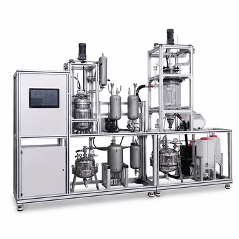
How Can Liquid-Liquid Mixing Pilot Plants Be Used To Quantify Mixing Efficiency With Bourne Reactions?

Competitive chemical test reactions, such as the Bourne network, offer a direct and quantitative method to assess mixing efficiency in pilot-scale liquid–liquid systems.
You run a carefully chosen set of reactions where a fast, diffusion-controlled step and a much slower step compete for a common reagent. When mixing is perfect, the fast reaction consumes the limiting reactant instantly, and the slow side reaction is effectively shut down. In a real stirred vessel, imperfect mixing creates local concentration spikes that allow the slow reaction to proceed, producing a measurable byproduct – such as methanol in the fourth Bourne reaction. By tracking that byproduct concentration across different agitation speeds, feed positions, or reactor geometries in a pilot plant, you can back-calculate a mixing time and rank configurations by their ability to sustain selective chemistry.

A liquid–liquid mixing pilot plant turns the subjective feel of “good mixing” into a hard number. Competitive reaction networks convert microscopic fluid dynamics into a quantifiable byproduct yield, directly linking reactor design and operating conditions to chemical selectivity. The result is a reproducible metric – often a characteristic mixing time – that guides scale-up decisions for fast, mixing-sensitive processes.

How a Competitive Reaction Quantifies What We Cannot See

The core idea is simple: let chemistry act as a molecular-scale probe of the fluid’s ability to blend.
You design a reactive system where one reaction is instantaneous (or nearly so) and another is kinetically limited. The instantaneous reaction is your baseline – it will go to completion as long as reagents meet. The slow reaction acts as a defect indicator: it can only happen where local hot spots of the limiting reagent survive long enough to react instead of being neutralized by the fast scavenger.

The Classic Example: The Fourth Bourne Reaction

The fourth Bourne system encapsulates this perfectly. An aqueous stream containing sodium hydroxide (NaOH) and hydrochloric acid (HCl) is brought into contact with an organic phase that holds 2,2-dimethoxypropane (DMP). Two reactions compete for the acid:

Fast, instantaneous: Neutralization of HCl with NaOH to form salt and water.
Slow, acid-catalyzed: Hydrolysis of DMP to acetone and methanol.

Under ideal, instantaneous mixing, every molecule of HCl meets NaOH and is consumed before it can encounter DMP. No methanol is formed.
Where mixing is sluggish, small eddies rich in HCl can persist. In those micro‑zones, the hydrolysis reaction gets a chance to run, yielding measurable methanol. The worse the mixing, the higher the methanol concentration in the product stream.

Why a Pilot Plant Matters

A benchtop beaker can demonstrate the principle, but a pilot plant introduces the real-world complexities that matter for scale-up: power-per-volume ratios, feed pipe locations, impeller type, baffle geometry, and continuous-flow dynamics. By systematically changing these variables and measuring the byproduct of the same competitive reaction, you create a direct, apples-to-apples map of mixing efficiency across different equipment configurations and scales.

From Byproduct Measurement to a Mixing Time

The real power of the method is not just knowing that a configuration is “better” – it’s in extracting a numerical mixing time that can be plugged into process models.

Running the Pilot-Scale Experiment

In a typical pilot run, the two liquid phases are fed continuously or as a semi-batch charge. Key steps include:

Fix the reaction recipe – concentrations, phase ratios, and stoichiometry are held constant so the competition only reflects fluid dynamics.
Vary the agitation intensity – measure byproduct (e.g., methanol via gas chromatography or online spectroscopy) at several impeller speeds, from just-off-the-bottom to fully dispersed.
Vary the geometry – test different impeller types, baffle arrangements, or feed point locations. A submerged feed near the impeller often yields far lower byproduct than a feed at the liquid surface.
Record process-relevant conditions – power input, holdup, drop size distribution – so that any change in byproduct can be correlated with a specific mixing variable.

Calculating Mixing Time from Selectivity

The competitive reaction network acts like a stopwatch for the fluid’s blending rate. With known kinetic constants for the slow reaction, a simple mass‑balance model can translate the measured byproduct yield into an apparent mixing time:

At high agitation, yield approaches zero, and mixing time is far shorter than the characteristic reaction time of the slow step.
As agitation drops, byproduct rises, and the model yields a longer mixing time because the fluid needs more time to eliminate concentration gradients.

You end up with a curve of mixing time vs. power input – a direct engineering criterion. Two geometries that draw the same shaft power can be compared head-to-head: the one that delivers the shorter mixing time at a given specific power is the better mixer for fast, selectivity‑driven reactions.

Practical Considerations for a Pilot Plant Campaign

Turning the Bourne reaction (or an analogous system) into a robust pilot protocol requires attention to the analytical and operational details.

Measuring the Byproduct Accurately

The slow reaction’s product – methanol in the fourth Bourne reaction, or ethanol/sodium chloride in other variants – must be quantified precisely at low levels.
Gas chromatography (GC) is the gold standard, often with a headspace or direct aqueous injection method. The detection limit directly influences the smallest mixing time you can resolve. For pilot plants targeting very intense mixing, you may need to push analytical sensitivity or adjust reagent concentrations to keep the byproduct signal above the noise floor.

Keeping the System Safe and Representative

The Bourne reactions often involve corrosive or hazardous chemicals (HCl, NaOH, organic solvents). Pilot plants need proper materials of construction and scrubbed vents.
Moreover, the test should mimic the physical properties of your real process fluids as closely as possible. Differences in interfacial tension, viscosity ratio, and density can shift drop breakage and coalescence behavior, altering the apparent mixing time. A Bourne test gives you a ranking of mixing hardware; it may not give you the exact absolute mixing time for a completely different chemical system unless you adjust the recipe to match key dimensionless groups like the Weber number.

Understanding the Trade-offs

Competitive reaction networks are a powerful diagnostic, but they are not a one‑size‑fits‑all solution.

The Analytical Bottleneck

Off‑line GC samples take time, limiting how rapidly you can scan a parameter space. Online spectroscopic methods (e.g., near‑infrared or Raman) can accelerate this, but they require careful calibration in a multiphase, often opaque pilot environment. Time spent on analysis is time not spent generating process insights.

Separating Micromixing from Mesomixing

A single Bourne experiment lumps together micromixing (molecular diffusion at the smallest scales) and mesomixing (larger‑scale circulation, feed plume dispersion). If your goal is to isolate a specific mixing regime, you may need multiple test reactions with different characteristic times or a more elaborate reactive tracer protocol. The standard Bourne test excels at capturing overall blending, but do not assume it always isolates the bottleneck you intend to fix.

Reagent Cost and Waste Streams

Running a competitive reaction continuously generates a waste stream – typically an aqueous salt solution contaminated with organic byproducts. At pilot scale, even a few hours of operation can require significant neutralization and disposal efforts. This is manageable, but it must be budgeted into the experimental plan.

Making the Right Choice for Your Goal

How you deploy a competitive reaction pilot study depends on what problem you are solving. Here is how to align the method with your objective:

If your primary focus is optimizing reactor hardware for a fast, mixing-sensitive reaction: Run a Bourne‑type test on at least three impeller types and two feed locations. Plot mixing time vs. P/V and select the configuration that minimizes mixing time at your target specific power.
If your primary focus is troubleshooting an existing plant where selectivity is below design: Reproduce the plant’s feed geometry and phase ratios in a pilot‑scale Bourne study. Map the current operating point and identify the agitation or baffle change that brings mixing time down to the required threshold.
If your primary focus is teaching or conveying the importance of mixing to a wider team: The Bourne reaction’s visual link between methanol concentration and mixing quality creates an unforgettable demonstration. The quantitative mixing time then connects the classroom to the control room.
If your primary focus is transferring a micro‑ or bench‑scale process to a commercial reactor: Use the pilot‑scale competitive reaction as a bridging step. Match the dimensionless mixing times (e.g., macro‑mixing time over reaction time) from small to large scale, and use the pilot plant to validate that the large‑scale hardware can deliver the same selectivity.

A well‑designed liquid–liquid mixing pilot plant doesn’t just tell you that one mixer is better than another – it hands you a numerical mixing time that lets you engineer selectivity with confidence.

Summary Table:

Aspect	Details for Bourne Reaction Network
Primary Application	Quantifies micro- and mesomixing in liquid-liquid systems
Competing Steps	Fast neutralization (HCl + NaOH) vs. slow hydrolysis (DMP + acid)
Key Byproduct	Methanol (measured via Gas Chromatography or online spectroscopy)
High Byproduct Yield	Indicates poor mixing (local acid concentration spikes persist)
Low Byproduct Yield	Indicates excellent mixing (rapid neutralization shuts down side reaction)
Engineering Value	Translates chemical selectivity into a standardized mixing time ($t_m$)

Ready to optimize your mixing processes and achieve predictable scale-up? LABPARK provides state-of-the-art Educational and Vocational Unit Operations Pilot Plants in chemical engineering, bioprocess & biotech, and environmental & water treatment. Designed specifically for universities, research institutes, and enterprises, our pilot systems empower you to quantify mixing efficiency and reaction dynamics with absolute precision.

Contact LABPARK today to discover how our custom pilot plant solutions can elevate your research and training capabilities!