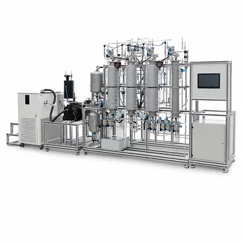
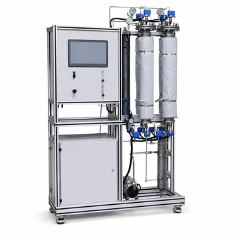
How To Configure Pilot Plants To Verify Two-Phase Flow Pressure Drop Calculations?

The key to verifying two-phase flow pressure drop lies in breaking the total loss into measurable components and comparing them against theory. A pilot plant configured with modular piping, multiple pressure sensors, and transparent test sections lets you isolate frictional, elevation, and fitting/exits losses. By measuring flow rates and mixture properties, you compute the two‑phase Reynolds number and fanning friction factor, then validate the calculations by matching them to real‑time sensor readings from the unit.

The most trustworthy verification comes from decomposing the total pressure drop—friction in straight pipe, hydrostatic head change, and sudden losses at exits—and confirming that each component follows the assumed high‑turbulence, mixture‑based model. Before applying the standard two‑phase correlation, you must first check that the mixture Reynolds number exceeds 200,000; otherwise, the empirical friction factors and phase‑distribution assumptions rapidly lose accuracy.

Configuring the Pilot Plant for Two‑Phase Pressure Drop Studies

Modular Piping Layouts That Isolate Each Loss Term

A verification‑ready pilot plant uses a straight horizontal test section of known length and diameter to capture friction loss.
Downstream, an inclined segment or a vertical riser introduces an elevation change whose hydrostatic contribution you can calculate separately.
Finally, the pipe discharges through a sharp‑edged exit into a larger vessel (e.g., a fractionation column), creating a distinct fitting loss you model with a loss coefficient.

Selecting Instrumentation and Materials

Equip long straight runs with high‑precision differential pressure transmitters tapped at multiple points, avoiding regions where flow is developing.
Swap in pipes of different absolute roughness (drawn tubing vs. steel) to observe how wall texture alters the two‑phase friction factor, mirroring single‑phase Moody‑diagram experiments with mixture properties.

Incorporating Gas‑Liquid Mixing and Flow Measurement

A precisely controlled gas and liquid injection system upstream establishes a known flow quality and mass flux.
Coriolis or magnetic flowmeters give total mass flow; a separate gas rotameter and liquid meter allow you to back‑calculate the in‑situ liquid volume fraction.

The Three Components of Total Pressure Loss

Straight Pipe Friction Loss

Calculate the mixture velocity from total volumetric flow rate and pipe cross‑section.
Estimate the mixture density and mixture viscosity from the liquid fraction using standard homogeneous‑flow assumptions.
With these, compute the mixture Reynolds number and obtain the two‑phase Fanning friction factor (from correlations or a two‑phase Moody chart). The expected pressure drop across the straight section is then (\Delta p_{\text{friction}} = 2f_{\text{TP}}\frac{L}{D}\rho_{\text{mix}} u_{\text{mix}}^2).

Elevation (Hydrostatic) Loss

In a vertical or inclined segment, the static head change follows (\Delta p_{\text{elev}} = \rho_{\text{mix}} g \Delta z).
Measure the true hydrostatic column between two accurately leveled pressure taps to isolate this term from friction.

Fitting and Exit Losses

A sharp‑edge exit into a column introduces a contraction‑like loss. The two‑phase pressure drop across the exit is often modeled with a multiplier on the single‑phase velocity head: (\Delta p_{\text{exit}} = K \frac{\rho_{\text{mix}} u_{\text{mix}}^2}{2}), where (K) typically falls near 1.0 for a sharp‑edged discharge.
Validating this term separately teaches how phase‑separation effects at vessel interfaces can dominate local pressure gradients.

Verifying Flow Regime Before Calculations

The Critical 200,000 Reynolds Number Threshold

The standard two‑phase summation method—friction, elevation, fitting losses—assumes fully turbulent flow with a mixture Reynolds number ≥ 200,000.
If the calculated (Re_{\text{mix}}) is lower, the empirical correlations for friction factor and phase holdup lose validity, and the measured vs. predicted agreement will degrade sharply.

Calculating Mixture Properties Correctly

First, determine the in‑situ liquid volume fraction from the measured phase velocities or from a slip‑model correlation.
From that fraction, weight the liquid and gas properties: (\rho_{\text{mix}} = \rho_L \lambda + \rho_G (1-\lambda)), and similarly for viscosity.
Compute (Re_{\text{mix}} = \frac{\rho_{\text{mix}} u_{\text{mix}} D}{\mu_{\text{mix}}}). Only if this number clears 200,000 can you confidently proceed with the three‑component breakdown.

From Theory to Verification: A Step‑by‑Step Approach

Isolate and Measure Each Component

Run the plant at steady gas and liquid flow rates, and record the total pressure drop across the entire piping complex.
Then, take differential readings across the horizontal test section only, across the vertical rise, and finally between the last pipe tap and the column vessel, effectively parting out the total loss.

Compare Calculated and Measured Component Sums

For the straight section, plug the measured flow data into the two‑phase friction factor and pipe geometry and compute (\Delta p_{\text{calc}}). Plot this against the measured value.
For the exit, use the known velocity head and a loss coefficient; for the elevation term, compute the hydrostatic head separately.
Add the three calculated (\Delta p) terms and compare the sum with the total pressure drop sensor, verifying that the decomposition accounts for all significant losses.

Run a “Regime‑Sensitivity” Experiment

Deliberately lower the flow until (Re_{\text{mix}}) drops below 200,000. Show that the same calculation procedure now systematically over‑ or under‑predicts the pressure drop, forcing a discussion on why two‑phase flow models are flow‑regime dependent.

Understanding the Trade‑offs

Simplifications That Limit Accuracy

Homogeneous‑mixture models ignore slip between phases, so they work best when the gas and liquid traverse the pipe at similar velocities—typically at high turbulence and dispersed flow.
When stratified or slug flow appears, the phase distribution contradicts the mixture‑viscosity blending rule, and errors become significant.

Instrumentation and Scale‑up Pitfalls

Differential pressure transmitters in two‑phase flow can be affected by liquid slugs or gas pockets that distort readings; careful tapping and purging are essential.
Pilot‑plant diameters are often small, which magnifies wall shear and makes roughness effects more pronounced than in industrial‑scale lines. Always discuss the scaling cautions when extrapolating to larger pipes.

Making the Right Choice for Your Goal

If your primary focus is educational demonstration: Use transparent PVC piping with a sharp‑edged exit into an open column, and run air‑water mixtures at high flow rates to stay above the Re = 200,000 threshold, making the pressure drop components visually and numerically clear.
If your primary focus is research validation: Include interchangeable test sections with varied roughness and multiple diameter sizes, and measure gas‑liquid holdup independently with gamma‑densitometry or quick‑closing valves to critically test the homogeneous mixture assumption.
If your primary focus is training for plant operations: Build in a “what‑if” scenario that requires using the verified model to perform an operational calculation—predicting how a change in fluid viscosity or flow rate will alter the total pressure loss, then test that prediction on the pilot plant.

Verifying two‑phase pressure drop calculations is about designing a system that transparently separates the governing physics into discrete, measurable contributions—and then having the discipline to confirm that the flow regime matches the model’s fundamental assumptions before trusting the numbers.

Summary Table:

Loss Component	Governing Physics / Model	Pilot Plant Instrumentation
Friction Loss	Fanning friction factor (requiring Re >= 200,000)	Straight horizontal test section, DP transmitters
Elevation Loss	Hydrostatic static head (density * g * height)	Vertical riser or inclined pipe, leveled taps
Exit Loss	Discharge loss coefficient (K ~ 1.0)	Sharp-edged discharge into a fractionation column

Bring Fluid Dynamics to Life with LABPARK

Are you looking to bridge the gap between theoretical calculations and physical process reality?

LABPARK provides premium Educational and Vocational Unit Operations Pilot Plants in chemical engineering, bioprocess & biotech, and environmental & water treatment. Designed specifically for universities, research institutes, and enterprises, our modular systems enable users to:

Isolate & Verify Physics: Easily separate friction, elevation, and exit losses with precise instrumentation.
Customize Configurations: Swap piping materials, adjust roughness, and introduce multi-phase mixtures.
Enhance Hands-On Learning: Provide students and researchers with industry-grade, transparent test setups.

Ready to upgrade your laboratory or training facility? Contact our engineering experts today to design your custom pilot plant solution!