How Are Porous Electrodes Modeled In Electrochemical Unit Operations Training Equipment? Macrohomogeneous Math

The core of modeling porous electrodes in training equipment lies in a deliberate simplification. Instead of mapping every convoluted pore, the mathematical model uses a macrohomogeneous, volume-averaged framework. This approach treats the electrode as two overlapping continuous phases—a solid matrix and a liquid electrolyte—defined by bulk-average properties like porosity and specific interfacial area. Material balance equations are then volume-averaged to reveal how concentration and potential evolve along the bed's length, giving students a powerful, intuitive tool for analyzing electrochemical reactors.

In educational electrochemical equipment, the complex pore structure is mathematically abstracted into measurable average parameters. This trades microscopic precision for macroscopic clarity, letting students focus on the dominant phenomena of mass transfer, ohmic drop, and reaction distribution without getting lost in geometric noise.

The Philosophy Behind the Volume-Averaged Model

The intricate, random geometry of a porous electrode—packed beds, felts, or sintered structures—presents a chaotic boundary condition problem. Solving it directly is computationally prohibitive and, for teaching, conceptually obstructive. The volume-averaged method collapses that complexity into a manageable form by redefining the system at a scale larger than individual pores but smaller than the entire reactor.

The Two-Phase Superposition

The model does not track separate solid chunks and liquid pockets. It imagines each point in space as being simultaneously occupied by both the solid matrix and the solution phase.

Each phase is continuous, and their interactions are described through exchange terms. This superposition eliminates the need to define a moving, irregular pore wall boundary. Instead, the geometry is encoded in two averaged scalar fields: porosity and specific surface area.

Porosity and Specific Interfacial Area

Porosity (ε) is the fraction of the bed's total volume that is void and filled with electrolyte. It quantifies how much space is available for ionic transport and flow.

Specific interfacial area (a) is the surface area of the pore walls per unit volume of the electrode. This single number captures the available site density where the electrochemical reaction physically occurs. Instead of tracing individual pore surfaces, the model simply says: in each tiny volume element, there are "a" square meters of reactive solid wall.

These two parameters transform the messy pore network into a continuum description, making the mathematical treatment feasible and the physical insight immediate.

Building the Governing Equations

With geometry reduced to average parameters, the next step is to apply conservation laws not at a point in a pore, but over a representative elementary volume containing many pores. This yields macroscopic balances that govern how concentrations and potential vary along the flow direction.

The Volume-Averaged Material Balance

A plug-flow material balance for a reacting species in the electrolyte becomes:

[ \frac{d(\varepsilon v c)}{dz} = \varepsilon D_{eff} \frac{d^2 c}{dz^2} - a , k_m (c - c_s) ]

Here the first term is convective transport with superficial velocity (v), the second accounts for axial dispersion via an effective diffusivity (D_{eff}), and the third is the volume-averaged reaction term. The rate of mass transfer from the bulk solution to the pore wall is expressed as the product of the specific area (a) and a mass transfer coefficient (k_m), multiplied by the concentration driving force. This is the key bridge that connects the simplified geometric parameters to the electrochemical kinetics.

Ohmic Potential Drop and Current Distribution

For the solid matrix, Ohm’s law is applied in a volume-averaged sense:

[ \nabla \cdot (\sigma_{eff} \nabla \phi_s) = -a , i_n ]

The effective conductivity (\sigma_{eff}) incorporates the tortuosity and porosity of the solid phase. The source term is proportional to the specific interfacial area and the local normal current density (i_n). This equation, solved alongside a similar one for the electrolyte phase, gives the potential distribution and reveals where the reaction localizes along the bed.

Student-Ready Analysis

Training equipment leverages these equations to teach key concepts visually. Students measure outlet concentrations or potential probes along the bed and compare them to model predictions. They can immediately see how changing porosity shifts the utilization depth or how insufficient conductivity causes the reaction to concentrate only near the current collector.

Understanding the Trade-offs

The macrohomogeneous model's elegance is also its limitation. Every educator and user must recognize what is being sacrificed when the pore-scale world is smoothed out.

Limitations of the Averaging Assumption

The model assumes that all gradients within a representative volume are negligible compared to the macroscopic gradients along the bed. This falls apart when pore sizes are large or reaction rates are extremely non-uniform.

It also cannot intrinsically predict local hot spots, blocking by gas bubbles inside a single pore, or the precise influence of pore-neck geometries. These effects are lumped into empirical parameters like the effective diffusivity, mass transfer coefficient, and effective conductivity.

The Risk of Over-Interpretation

Students might mistakenly treat the model's predictions of "local" concentration as an actual pore-scale concentration. It is a phasic average—a smoothed field. The model is excellent for predicting integral performance (total conversion, overall potential drop), but it only provides a first-order estimate of the reaction environment at the pore wall.

Making the Right Choice for Your Educational Focus

The value of the macrohomogeneous approach is context-dependent. Here is how to align the method with your primary training objective.

If your primary focus is teaching core transport phenomena: Use the volume-averaged model to isolate how convection, migration, and diffusion interact with a distributed reaction. The clean mathematics keeps the physics visible and debuggable.
If your primary focus is linking design parameters to performance: Exploit the model's explicit dependence on porosity and specific area. This lets learners quantify the penalty of a denser bed (higher area, higher pressure drop) or the benefit of a higher-conductivity matrix.
If your primary focus is reinforcing experimental observation: Pair measured axial concentration profiles with model equations. The act of fitting an effective parameter, like the mass transfer coefficient, teaches scale-up principles without requiring pore-scale imaging.
If your primary focus is exploring fundamental assumptions: Challenge students to identify where the volume-averaged approach breaks down—near the current feeder, at low flow rates where dispersion dominates, or for very fast reactions limited by pore diffusion. This builds a critical mindset that every model has a domain of validity.

A well-designed training unit using the macrohomogeneous model doesn't hide complexity—it strategically defers it, giving engineers a mental framework that survives long after the details of a particular pore geometry are forgotten.

Summary Table:

Parameter	Physical Meaning	Role in Mathematical Model
Porosity (ε)	Fraction of bed volume filled with electrolyte	Determines space for ionic transport and flow velocity
Specific Interfacial Area (a)	Pore wall surface area per unit volume	Defines the density of active reaction sites
Effective Conductivity (σ_eff)	Adjusted conductivity accounting for tortuosity	Governs potential drop and current distribution

Bring Advanced Electrochemical Modeling to Life with LABPARK

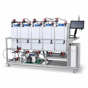
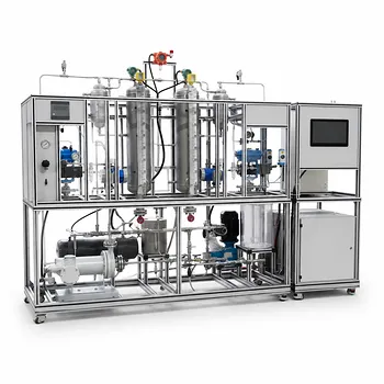
Looking to enhance your engineering curriculum or research capabilities? LABPARK provides state-of-the-art Educational and Vocational Unit Operations Pilot Plants in chemical engineering, bioprocess & biotech, and environmental & water treatment.

Our hands-on training systems help universities, research institutes, and enterprises bridge the gap between complex mathematical models—like volume-averaged porous electrode equations—and real-world physical measurements.

Ready to upgrade your laboratory? Contact LABPARK today to discuss your training equipment needs!