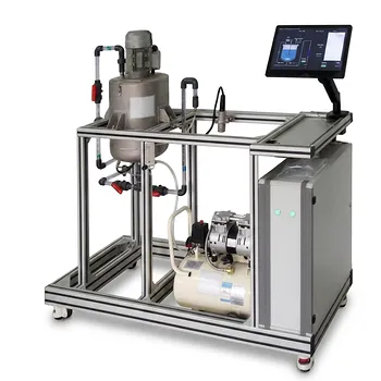
Fluid mixing unit operation pilot plants are used to test whether two or more continuous feed streams blend to the intended composition while satisfying component mass balances. Operators measure each inlet stream’s mass flow rate and composition, combine the streams under controlled mixing conditions, and analyze the outlet stream. At steady state, the measured outlet total and component mass flows are compared with the calculated inlet values to determine whether the balance closes.

A mixing pilot plant connects process behavior with mass-balance theory: correct stream blending requires accurate flow ratios, effective mixing, reliable composition measurements, and negligible unexplained accumulation.

How the Pilot Plant Represents Stream Blending

Establishing the Mixing System Boundary

The system boundary normally surrounds the feed lines, mixing vessel or inline mixer, and combined outlet. Streams entering the boundary are treated as inputs, while the blended product leaving it is treated as the output.

For steady-state operation without reaction, evaporation, leakage, or accumulation:

[ \sum \dot{m}{in} = \dot{m}{out} ]

where (\dot{m}) represents mass flow rate.

Combining Streams with Different Compositions

The plant feeds two or more fluids with different concentrations or mass fractions into a common mixing device. For example, one stream may contain a high solute concentration while another contains mostly solvent.

By adjusting pump speeds or control valves, operators vary the feed ratio and observe whether the blended outlet reaches the target intermediate specification.

Demonstrating Continuous Operation

Unlike a batch demonstration, a continuous mixing plant shows how composition evolves as the system starts up, approaches steady state, and responds to disturbances. This exposes the practical difference between a theoretical blend ratio and the composition actually delivered by equipment.

How Component Mass Balance Closure Is Calculated

Writing the Component Balance

For component (i), the steady-state balance is:

[ \sum_j \dot{m}j w{i,j,in}

\dot{m}{out} w{i,out} ]

Here, (w_i) is the mass fraction of component (i). With two inlet streams, the balance becomes:

[ \dot{m}1 w{i,1} + \dot{m}2 w{i,2}

\dot{m}{out} w{i,out} ]

If the streams contain a solute and solvent, the solute balance can be evaluated independently from the total mass balance.

Predicting the Target Outlet Composition

The expected outlet mass fraction is calculated from the inlet measurements:

[ w_{i,out,expected}

\frac{\dot{m}1 w{i,1}+\dot{m}2 w{i,2}} {\dot{m}_1+\dot{m}_2} ]

The measured outlet composition is then compared with this predicted value. Agreement indicates that the feed ratio and composition measurements are consistent with the intended blend.

Quantifying Balance Closure

A component balance closure can be expressed as:

[ \text{Closure}_i

\frac{\dot{m}{i,out}} {\sum_j \dot{m}{i,j,in}} \times 100% ]

A result near 100% indicates agreement between measured inlet and outlet component flows. The acceptable deviation depends on instrument accuracy, sampling uncertainty, operating stability, and the process itself.

What Operators Measure

Feed and Product Flow Rates

Flow meters or calibrated weighing methods provide the mass flow rate of each inlet stream and the combined outlet. Accurate flow data are essential because an error in one feed rate directly affects the predicted blend composition.

Operators also verify whether volumetric flow measurements can legitimately be converted to mass flow. Density changes, temperature, and concentration may make a simple volume-to-mass conversion inaccurate.

Stream Compositions

Samples from each inlet and the outlet are analyzed for the relevant component concentration or mass fraction. Depending on the fluid system, analysis may use laboratory assays, conductivity, density, spectroscopy, or another calibrated measurement method.

The inlet composition measurements establish the expected outlet composition; the outlet measurement tests whether the physical system achieved it.

Mixing and Operating Conditions

The plant may record vessel level, agitator speed, motor torque, power consumption, temperature, and residence time. These variables help determine whether the observed composition reflects the intended steady-state process.

Transparent vessels and interchangeable agitators can also make circulation patterns and mixing limitations visible. Inline static mixers may be compared with stirred tanks to study how equipment configuration affects blending performance.

How the Demonstration Identifies Process Problems

Detecting Incorrect Feed Ratios

If the outlet composition differs from the calculated target, the first checks are usually the measured flow rates, valve positions, pump calibration, and stream concentrations. A mismatch may indicate that one stream is entering at a different rate than assumed.

This makes the pilot plant useful for validating feed-ratio control before applying the strategy to a commercial process.

Identifying Incomplete Mixing

A poorly mixed outlet can produce variable samples even when the average flow rates are correct. Concentration differences between samples taken at different times or locations may indicate short-circuiting, stagnant regions, inadequate agitation, or insufficient residence time.

A single outlet sample can conceal this problem, so repeated sampling and evaluation of time variation are important.

Separating Measurement Error from Process Error

A balance that does not close does not automatically prove that material has disappeared. Sampling bias, analyzer calibration, flow-meter error, density assumptions, and changes in holdup can all create apparent imbalance.

Operators therefore compare replicate samples, confirm instrument calibration, and wait for stable flow, level, and composition before judging closure.

Why Steady State Matters

Accounting for Accumulation

The general component balance is:

[ \text{Input} - \text{Output}

\text{Accumulation} ]

During startup or a change in operating conditions, material can accumulate in the vessel or connected piping. In that period, inlet and outlet component flows are not expected to match immediately.

At steady state, the accumulation term is approximately zero, allowing the simpler input-output comparison.

Establishing a Reliable Test Period

A useful balance requires a defined operating window during which flow rates, levels, and compositions remain sufficiently stable. Operators collect multiple measurements during that period rather than relying on a single instantaneous reading.

Averaging the data can reduce random measurement variation, while the spread of the results reveals process instability.

Understanding Residence-Time Effects

The outlet composition may lag behind a change in inlet conditions because material must pass through the mixing volume. This delay is governed by the effective residence time and mixing behavior.

The pilot plant therefore demonstrates both the final steady-state blend and the dynamic response of the process.

Connecting Mixing Quality to Process Performance

Studying Laminar and Turbulent Mixing

By changing viscosity, flow rate, agitator speed, or mixer geometry, users can examine different flow regimes. These changes influence circulation, blend time, and the uniformity of the outlet composition.

Mixing studies may also relate power consumption to Reynolds number and Power number, supporting equipment comparison and scale-up analysis.

Evaluating Micro-Mixing and Feed Distribution

In systems involving fast reactions or multiple reactions, the local way in which streams contact one another can affect conversion and product distribution. Split-and-recombine devices, segmented feeds, and other mixer configurations allow users to examine these effects experimentally.

The component balance remains necessary, but it may not be sufficient to explain product quality when local mixing controls reaction behavior.

Validating Process Models

Measured flow rates and compositions can be compared with calculations from design models or process simulations. Differences help identify unrealistic assumptions about mixing, density, residence time, or control performance.

This empirical validation reduces uncertainty before a process is scaled to commercial equipment.

Understanding the Trade-offs

Total Balance Closure Does Not Prove Uniform Mixing

A total mass balance can close even when the outlet is compositionally nonuniform. Proper closure confirms conservation across the measured boundary; it does not by itself prove that every portion of the outlet has the same composition.

Spatially distributed sampling, time-series data, or tracer testing may be needed to evaluate uniformity.

More Instrumentation Increases Complexity

Additional flow meters, analyzers, sampling points, and data logging improve diagnosis but introduce more calibration requirements and possible failure modes. The measurement system must be treated as part of the experiment.

Poorly calibrated instruments can make a well-operated mixer appear to have a process defect.

Scale-Up Is Not Direct

A pilot mixer can demonstrate blend behavior and reveal operating trends, but commercial equipment may differ in geometry, residence-time distribution, fluid properties, and energy input. Matching agitator speed alone is generally not enough to guarantee equivalent performance.

Pilot data should therefore be interpreted using appropriate scale-up criteria and process objectives.

Steady-State Testing Can Miss Transients

A steady-state balance may show excellent closure while startup, shutdown, feed switching, or control disturbances cause unacceptable off-specification material. A complete evaluation includes both stable operation and relevant operating transitions.

Making the Right Choice for Your Goal

A mixing pilot plant is most valuable when its measurements are designed around the decision the process must support.

If your primary focus is target blend composition: Measure every inlet flow and composition, calculate the expected outlet mass fraction, and verify it with repeated product samples.
If your primary focus is mass balance closure: Define the system boundary, measure total and component mass flows, and evaluate closure only after steady-state conditions are established.
If your primary focus is troubleshooting: Compare measured feed ratios, outlet variability, mixing conditions, and instrument calibration before attributing imbalance to the mixer.
If your primary focus is equipment selection or scale-up: Test relevant viscosities, flow regimes, mixer configurations, and residence times while recording both composition uniformity and mixing power.
If your primary focus is process control: Introduce controlled changes in feed rate or composition and measure the resulting outlet response, including the transport delay through the mixing volume.

A well-designed fluid mixing pilot plant turns stream blending and mass balance closure into measurable evidence for process design, control, troubleshooting, and scale-up.

Summary Table:

Key Area	What the Pilot Plant Demonstrates
System boundary	Defines inlet streams, mixing equipment, and the combined outlet
Stream blending	Tests whether feed ratios produce the intended outlet composition
Component balance	Compares inlet component flows with measured outlet flows
Steady-state testing	Minimizes accumulation effects for reliable closure calculations
Process measurements	Uses flow, composition, density, temperature, level, and residence-time data
Troubleshooting	Identifies feed-ratio errors, incomplete mixing, sampling bias, and instrument issues
Scale-up support	Compares mixer configurations, flow regimes, residence times, and power requirements
Process control	Evaluates outlet response to feed changes and operating disturbances

Need to verify stream blending, improve mass balance closure, or reduce scale-up risk? Contact LABPARK to discuss an Educational or Vocational Unit Operations Pilot Plant tailored to your objectives. LABPARK provides fluid mixing and related pilot plants for chemical engineering, bioprocess and biotechnology, and environmental and water treatment applications. Universities, research institutes, and enterprises can use our systems to measure flow and composition, evaluate mixing performance, validate process models, train operators, troubleshoot imbalance, and generate reliable data for equipment selection and commercial process design.