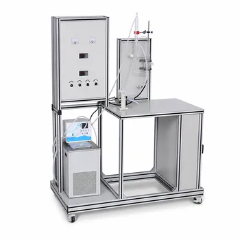
The single reduced temperature of 0.7 is not an arbitrary choice—it is the universal benchmark that separates simple fluids from complex ones. Vapor pressure data near this point is critical because it directly defines the acentric factor (ω), the key third parameter used to calibrate cubic equations of state for non‑ideal molecules. In a pilot plant, measuring vapor‑liquid equilibrium around this characteristic temperature allows engineers to anchor thermodynamic models to reality and observe exactly how a single, well‑chosen data point governs the accuracy of separation predictions across an entire unit operation.
Because the reduced vapor pressure at Tr = 0.7 reflects a molecule’s non‑ideal shape and polarity far from the critical point, it provides the empirical anchor for the acentric factor. Calibrating a thermodynamic model to this one condition—validated by a pilot‑scale distillation or VLE measurement—directly determines the reliability of the phase‑equilibrium calculations that underpin the majority of all chemical engineering data requests.
Why a Single Temperature Carries So Much Weight
The Molecular Fingerprint Captured at Tr = 0.7
Near the critical point, all fluids behave similarly; vapor‑pressure curves converge and molecular individuality is masked.
At a reduced temperature of 0.7—well below the critical region—simple spherical molecules (argon, krypton) exhibit a reduced vapor pressure of roughly 0.1, giving an acentric factor of zero.
Complex molecules with dipole moments, non‑spherical shapes, or hydrogen‑bonding capability deviate strongly from this baseline at the same reduced temperature. That deviation is exactly what the acentric factor quantifies, making Tr = 0.7 a high‑contrast fingerprint of molecular structure.
How One Point Calibrates an Entire Equation of State
Cubic equations such as Soave‑Redlich‑Kwong and Peng‑Robinson use ω to tune the temperature‑dependent alpha function, which shapes the entire predicted vapor‑pressure curve.
When ω is anchored by reliable data at Tr = 0.7, the entire saturation envelope—from triple point to critical point—is pulled into alignment. An error at this single temperature propagates into bubble‑point pressures, dew‑point temperatures, and K‑values throughout the column.
It is this “single‑point leverage” that makes vapor pressure at Tr = 0.7 the most influential piece of pure‑component data in process simulation.
How a Pilot Plant Turns Theory into Proof
Seeing the Acentric Factor’s Impact on a Running Column
A distillation pilot plant makes the abstract parameter tangible. By setting a fixed feed and operating pressure, the observed top and bottom compositions directly reflect the underlying vapor‑liquid equilibrium.
When the simulation uses a default‑databank acentric factor that is slightly off, the predicted column temperature profile, reflux ratio, and product purities will drift away from the plant readings. This discrepancy is often the first and clearest sign that the model’s core pure‑component anchor needs attention.
Tuning ω—even by a few percent—can bring the simulation back into line, vividly demonstrating that no amount of tray‑efficiency adjustment can compensate for a foundational error in vapor‑pressure behavior around Tr = 0.7.
Building a Calibration Workflow from Plant Data
In a teaching or R&D pilot plant, you can measure phase equilibrium directly: sample liquid and vapor from equilibrium cells or draw tray samples for analysis.
By plotting the measured relative volatilities against model predictions, the region near Tr = 0.7 becomes a diagnostic hotspot. A consistent bias there signals an incorrect acentric factor, while good agreement confirms the model’s structure is sound.
Many practitioners then use this validated ω to regress binary interaction parameters for complex mixtures—fixing the pure‑component anchor first, then fine‑tuning the mixture rules—a sequence that preserves physical meaning and yields robust scale‑up predictions.
Practical Workarounds When Direct Measurement Is Unavailable
Not every pilot‑plant fluid can be safely or practically brought to a reduced temperature of 0.7. In those cases, the acentric factor can be estimated from readily available data using Edmister’s formula:
ω = (3/7) * [θ/(1‑θ)] * log₁₀(P_c) – 1, where θ = T_n/T_c.
A pilot plant still adds value even with an estimated ω: if the column’s measured bubble‑point temperature or overhead composition agrees with predictions that use the estimated value, you gain confidence. If it does not, you have clear guidance to measure the missing vapor‑pressure point or seek a more accurate experimental ω.
Understanding the Trade‑offs and Pitfalls
A single‑point characteristic can never capture the full complexity of strongly associating fluids. For mixtures dominated by hydrogen bonding, activity‑coefficient models (NRTL, UNIQUAC) may be required, and the acentric factor becomes one of many parameters rather than the main knob.
Pilot‑plant measurements are not immune to error: poor temperature control, sub‑cooling, or mass‑transfer resistance can mask the true VLE signature. An operator must be careful not to “correct” an accurately estimated ω because of a column efficiency problem.
Relying solely on simulation databases without cross‑checking against experimental data is a known risk. Third‑party databanks sometimes contain regressed acentric factors that were never verified at Tr = 0.7 for the specific compound, leading to model mismatch that a pilot plant will immediately reveal.
Finally, the acentric factor is a pure‑component property. It provides the best foundation, but for multicomponent systems the real test is whether the chosen mixing rules and interaction parameters carry that accuracy forward. Pilot plants expose the whole chain, from single‑molecule descriptor to column performance.
Making the Right Choice for Your Goal
- If your primary focus is pure‑component characterization: Measure or source a reliable vapor‑pressure value at Tr = 0.7—or, when measurement is impossible, use Edmister’s method—to anchor your cubic equation of state. A pilot‑scale ebulliometer or equilibrium cell provides the highest confidence.
- If your primary focus is troubleshooting a distillation pilot plant: Start by comparing simulated temperature and composition profiles with live data. Verify the acentric factor’s accuracy first; only after that, adjust binary interaction parameters. This ordering prevents false corrections that would fail at scale‑up.
- If your primary focus is strengthening chemical engineering education: Let students operate a pilot column with a simulated acentric factor deliberately offset by 10–15%. The resulting shift in overhead purity and reflux demand cements the lesson that one critical thermophysical number can control an entire unit operation—and that “approximately right” data at Tr = 0.7 is far more valuable than “precisely wrong” correlations.
Keep the single data point at Tr = 0.7 as your model’s anchor, test it on the pilot plant, and you will own a calibration that travels reliably from bench‑scale curiosity to full‑scale design.
Summary Table:
| Key Concept | Significance at Tr = 0.7 | Pilot Plant Application & Validation |
|---|---|---|
| Acentric Factor (ω) | Quantifies molecular shape and polarity deviation from simple spherical fluids. | Anchors cubic equations of state (SRK, Peng-Robinson). |
| Model Calibration | Shapes the predicted vapor-pressure curve across the entire saturation envelope. | Direct VLE measurements verify the accuracy of phase-equilibrium models. |
| Unit Operations | Governs bubble points, dew points, and component K-values in simulation. | Exposes discrepancies between simulated profiles and actual column data. |
Bring Thermodynamic Theory to Life with LABPARK
Are you looking to bridge the gap between complex thermodynamic modeling and real-world chemical engineering? LABPARK provides high-quality Educational and Vocational Unit Operations Pilot Plants in chemical engineering, bioprocess & biotech, and environmental & water treatment.
Designed specifically for universities, research institutes, and enterprises, our pilot plants enable hands-on calibration of equations of state, direct verification of VLE data, and practical troubleshooting of distillation columns.
Don't let modeling discrepancies derail your process scale-up or educational curricula. Contact LABPARK today to discover how our tailored pilot plant solutions can elevate your research and training capabilities!
Related Products
- Binary System Vapor Liquid Equilibrium Data Determination Educational Unit Operations Pilot Plant
- Circulating Wind Tunnel Drying and Convective Heat Transfer Coefficient Determination Educational Pilot Plant
- Bernoulli Equation Demonstration Unit Operations Pilot Plant
- Two Phase Flow Pattern Velocity Resistance Measurement Educational Pilot Plant
- Educational Unit Operations Pilot Plant for Intraparticle Diffusion Effective Factor Measurement
People Also Ask
- For VLE Experiments: Fugacity vs. Activity Coefficient Method Selection Criteria
- Why correlate VLE pilot plant data using Wilson, NRTL, and UNIQUAC? Achieve Accurate Column Scale-Up
- How do pilot plants assist in teaching & researching non-ideal VLE? Bridge Theory & Physical Validation
- How to Model VLE for Supercritical & Unstable Components? Pilot Plant Methods
- Why is accurate VLE data critical? Optimize Unit Operations & Process Scale-Up