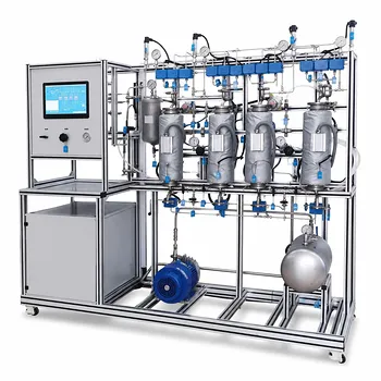
What Equations Govern Mass Balance & Reaction Kinetics In A Non-Isothermal Cstr?

The equations that govern the reactant in a non‑isothermal CSTR training system are the dynamic component mass balance and the Arrhenius expression for the rate constant.
For a constant‑density liquid‑phase reaction, the mole balance on reactant P is d(Cp)/dt = (F/V)(Cp0 – Cp) – k * Cp^n, where Cp is the outlet concentration, F the volumetric flow, V the reactor volume, and n the reaction order. The temperature‑dependent rate constant k is given by k = k0 * exp(–Ea/(RT)). Because temperature is intentionally varied, you also need an energy balance to compute the temperature T that feeds the Arrhenius equation.

The core governing equations are a coupled set: a transient mass balance for the reactant, an Arrhenius law for the reaction rate, and an energy balance that captures the heat of reaction and heat exchange. In a training skid, these three equations are solved simultaneously to show how manipulating jacket temperature or feed conditions alters conversion and reaction rate.

The Mass Balance: Tracking Reactant Concentration

The CSTR is assumed to be perfectly mixed, so the outlet concentration equals the concentration inside the vessel at all times. The mass balance simply states that the accumulation of reactant equals what flows in minus what flows out minus what is consumed by reaction.

The General Form

For a liquid‑phase system with constant density and constant volume, the equation reduces to a familiar ordinary differential equation:
dCp/dt = (F/V)*(Cp0 – Cp) – r(Cp, T)

Here r(Cp, T) is the rate of disappearance of P, which is the product k * Cp^n for a power‑law model.

Variable Volume Cases

The primary reference gives the more general form d(V*Cp)/dt = F0*Cp0 – F*Cp – V*k*Cp^n. This handles situations where inlet and outlet flows differ—important if you are training operators on startup, shutdown, or fed‑batch transitions where volume is not constant.

Reaction Kinetics: How Temperature Drives the Rate

The reaction rate term is where the non‑isothermal character enters. The specific rate constant k is not a fixed number; it depends exponentially on absolute temperature.

The Arrhenius Equation

k = k0 * e^(–Ea/(R*T))

k0 (pre‑exponential factor) sets the maximum possible rate at infinite temperature.
Ea (activation energy) determines how sharply the rate rises with temperature.
A high Ea means a small temperature change can dramatically alter the reaction speed.

In a training system, students often change the jacket setpoint and watch how k—and therefore conversion—responds. The Arrhenius law is the mathematical bridge that gives the experiment its predictive power.

Why an Energy Balance Is Indispensable

The mass balance and Arrhenius equation alone cannot model a non‑isothermal CSTR because they contain the unknown T. You must close the system with an energy balance:
d(ρ*V*cp_sol*T)/dt = F*ρ*cp_sol*(T0 – T) + UA*(Tj – T) + (–ΔH_rxn)*V*k*Cp^n

This equation accounts for sensible heat of the feed stream, heat transfer through the jacket (UA*(Tj–T)), and heat generated or consumed by the reaction. Together with the mass balance, it forms a coupled set that predicts the reactor’s thermal and concentration trajectory.

Understanding the Assumptions and Their Consequences

Training systems deliberately create a safe, idealized environment. The equations you use reflect those simplifications, and it is critical to recognise their limitations.

Perfect Mixing Is a Model Assumption

The CSTR model treats the entire volume as homogeneous. In reality, dead zones or short‑circuiting can occur, especially at low agitation speeds. When you use the ODE above, you assume the measured concentration is instantly representative of the whole tank.

Constant Density and Heat Capacity Are Approximations

Many liquid‑phase reactions generate only small density changes, so treating V and ρ as constant simplifies the math enormously. In training systems this is usually justified, but if the goal is to model highly exothermic polymerisations, you would need to include property variations.

Single‑Step Kinetics May Not Capture Real Complexity

The power‑law rate k*Cp^n is a convenient empirical fit. Real reactions often have intermediate steps or catalyst deactivation. A training unit designed to teach control and operations can still convey the essential coupling between temperature and rate using a simple kinetic form.

Applying the Equations in a Training Context

If Your Primary Focus Is Understanding Fundamentals:

– Use the constant‑volume mass balance and the Arrhenius equation to manually calculate steady‑state conversion at different jacket temperatures. This builds intuition for activation energy and residence time.

If Your Primary Focus Is Process Control Design:

– Simulate the full ODE system (mass + energy balance) to test PID tuning for jacket temperature. The non‑linear Arrhenius term turns even a simple CSTR into a challenging control problem.

If Your Primary Focus Is Operator Training:

– Use the equations as the invisible engine inside a dynamic simulator. The trainee sees realistic cause‑and‑effect—increase coolant flow, temperature drops, conversion falls—backed by the mass and energy balances.

You now have the exact set of equations that power a non‑isothermal CSTR training system: a dynamic mole balance, an Arrhenius‑driven rate constant, and an energy balance that ties them together. Master these, and you hold the key to predicting and controlling reaction behaviour under varying thermal conditions.

Summary Table:

Equation Type	Formula	Key Purpose
Mass Balance (Constant Volume)	`dCp/dt = (F/V)(Cp0 - Cp) - k Cp^n`	Tracks transient reactant concentration inside the reactor.
Arrhenius Kinetics	`k = k0 * exp(-Ea / (R * T))`	Calculates the temperature-dependent reaction rate constant.
Energy Balance	`d(ρVcpT)/dt = Fρcp(T0 - T) + UA(Tj - T) + (-ΔH_rxn)VkCp^n`	Tracks temperature changes from reaction heat and jacket exchange.

Bring Chemical Engineering Theory to Life with LABPARK

Understanding complex CSTR mathematical models requires hands-on experience. LABPARK provides premium Educational and Vocational Unit Operations Pilot Plants in chemical engineering, bioprocess & biotech, and environmental & water treatment.

Specially designed for universities, research institutes, and enterprises, our training systems enable students and operators to safely visualize mass balances, kinetic behavior, and process control in real time.

Ready to upgrade your training laboratory? Contact our engineering experts today to find the perfect pilot plant solution for your institution.