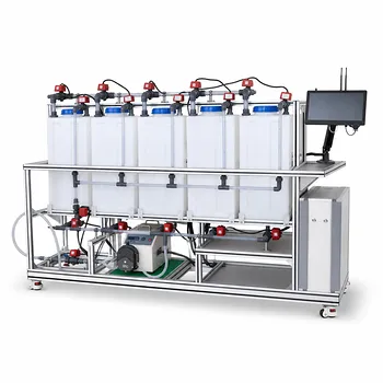
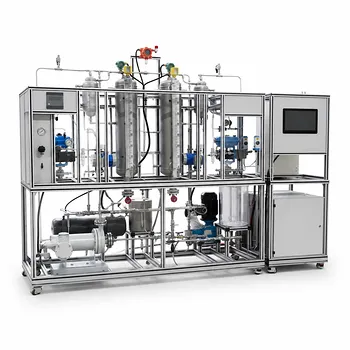
How Is The Steady-State Macroscopic Water Balance Equation Applied In Environmental And Water Treatment Pilot Plants? A Practical Guide

The steady-state macroscopic water balance is applied by equating all water entering a pilot plant system with all water leaving it. For an open hydrological or treatment pilot system, the balance is typically written as (R_1 + P = R_2 + E + W), where (R_1) is inlet flow, (P) is precipitation or an equivalent water addition, (R_2) is discharge, (E) is evaporation, and (W) is seepage, recharge, or other unmeasured loss. Because steady state assumes no net accumulation, the discharge can be calculated as (R_2 = R_1 + P - E - W).

A steady-state water balance turns a pilot plant into a controlled accounting system: measured inflows, outflows, evaporation, and seepage must reconcile when storage is constant. Differences between the calculated and measured values help quantify process losses, evaluate water recovery, and identify measurement or operating problems.

What the Balance Represents

Defining the System Boundary

The first step is to define exactly which part of the pilot plant is being analyzed. The boundary may include an entire open reservoir simulator, a treatment basin, a clarifier, a membrane unit, or the complete pilot process.

Every water stream crossing that boundary must be identified, including liquid feeds, treated effluent, sludge-associated water, evaporation, drainage, leaks, and seepage.

Applying the Steady-State Assumption

At steady state, the volume of water stored inside the defined system does not change with time. The general balance is:

[ \text{Accumulation} = \text{Inflows} - \text{Outflows} ]

Setting accumulation to zero gives:

[ \text{Total inflows} = \text{Total outflows} ]

This assumption is valid only after startup transients have passed and operating conditions such as flow rates, levels, and temperatures are reasonably stable.

Using the Macroscopic View

A macroscopic balance evaluates the pilot plant as a whole rather than describing flow at every point inside it. It does not require a detailed velocity or concentration profile within the equipment.

This makes it useful for checking overall performance, calculating an unknown stream, and comparing actual operation with the design basis.

How It Is Applied in a Pilot Plant

Listing and Measuring Water Inputs

Operators measure the primary inlet flow, (R_1), using a flowmeter, calibrated tank, weighing system, or timed-volume measurement. Other intentional additions, such as wash water or chemical solution, should also be included when they contribute materially to the water volume.

For an open system exposed to weather, precipitation (P) may be measured with a rain gauge and converted to a volume using the exposed surface area:

[ P = \text{rainfall depth} \times \text{surface area} ]

Quantifying Water Outputs

The discharge flow, (R_2), is commonly measured directly at the outlet. Measurement methods include inline flowmeters, weirs, flumes, pump calibration curves, or collection tanks.

Evaporation (E) may be estimated from water-level decline, mass loss from a covered weighing vessel, an evaporation pan, or a model using temperature, humidity, wind, and exposed area.

Accounting for Seepage and Recharge

Seepage or recharge, (W), represents water moving through the pilot plant boundary into or out of surrounding soil, gravel, liners, groundwater simulators, or drainage layers. It can be estimated using collection drains, underdrain flowmeters, lysimeters, or changes in measured system storage.

In a well-contained treatment unit, (W) may be negligible. It should still be stated as an assumption rather than silently omitted.

Solving for an Unknown Flow

Once the other terms are known, the missing stream is obtained algebraically. For discharge:

[ R_2 = R_1 + P - E - W ]

For example, if the inlet is known but discharge is difficult to measure accurately, measured precipitation, evaporation, and seepage can be used to estimate the expected outlet flow.

Conversely, if the outlet is measured, the balance can be rearranged to estimate evaporation or seepage:

[ E = R_1 + P - R_2 - W ]

The calculated value should then be compared with an independent measurement where possible.

Linking Water Balance to Treatment Performance

Separating Flow Accounting from Contaminant Accounting

The water balance tracks the quantity of water. A contaminant balance tracks a constituent such as BOD, nitrogen, phosphorus, suspended solids, or chlorine residual.

For a nonreactive constituent at steady state:

[ \sum Q_{\text{in}} C_{\text{in}} = \sum Q_{\text{out}} C_{\text{out}} ]

For a reactive treatment process, the balance must also include generation or consumption by reaction:

[ \text{Input} - \text{Output} + \text{Generation} - \text{Consumption} = 0 ]

A correct water balance therefore provides the flow basis needed for treatment-efficiency and pollutant-loading calculations.

Evaluating Mixing and Dilution

Pilot plants can simulate the effect of treated effluent entering a receiving stream. Under a complete-mixing assumption, the downstream concentration is:

[ C_{\text{downstream}} = \frac{Q_{\text{stream}}C_{\text{stream}}

Q_{\text{effluent}}C_{\text{effluent}}} {Q_{\text{stream}}+Q_{\text{effluent}}} ]

Researchers can vary the stream and effluent flow rates to examine dilution, downstream pollutant concentrations, and potential receiving-water impacts.

The result is a screening calculation, not a replacement for a detailed river model when mixing is incomplete, reactions occur, or conditions vary over time.

Supporting Chemical-Dose Calculations

A reliable water-flow measurement is also required for chemical dosing. For example, a target chlorine residual depends on the relationship between chemical mass feed rate and treated-water flow:

[ \text{Dose} = \frac{\text{chemical mass rate}}{\text{water volumetric flow rate}} ]

Using a consistent basis allows operators to convert between dosing units and concentration units such as milligrams per liter. This supports process control and water-quality verification.

Checking Water Recovery

Pilot plants often compare water entering the process with useful water recovered at the outlet. The balance identifies water lost through evaporation, sludge handling, membrane concentrate, drainage, or leaks.

A simplified recovery measure can be expressed as:

[ \text{Water recovery} = \frac{\text{usable recovered water}}{\text{water entering the system}} \times 100% ]

The exact definition should match the process objective and specify whether recycled internal streams are included.

Verifying the Balance in Practice

Establishing a Consistent Time Basis

All terms must use the same basis, such as liters per minute, cubic meters per day, or kilograms per hour. A rainfall depth cannot be added directly to a flow rate until it has been converted to volume per unit time.

For liquid water, volume and mass balances can often be related using density. At ordinary conditions, treating water density as constant is usually reasonable, but the assumption should be reviewed when temperature or composition varies significantly.

Creating a Stream Inventory

A process flow diagram should show every relevant inlet, outlet, recycle, drain, overflow, and loss pathway. Each stream should have a defined direction, measurement location, unit, and sampling or logging frequency.

This inventory prevents common omissions such as backwash water, chemical carrier water, sludge dewatering liquid, or bypass flow.

Collecting Synchronized Data

Flow, level, temperature, pressure, precipitation, and water-quality data should be recorded over the same operating period. Sensors should be calibrated, and readings should be checked against manual measurements or tank-volume tests.

A balance calculated from measurements taken at different times can appear inconsistent even when the plant is operating correctly.

Calculating the Closure Error

A useful verification metric is the balance closure error:

[ \text{Closure error} = \frac{\text{Total inflows} - \text{Total outflows}} {\text{Total inflows}} \times 100% ]

The acceptable range depends on the measurement uncertainty and the purpose of the experiment. A large unexplained error may indicate leakage, unmeasured evaporation, inaccurate flow instrumentation, changing storage, or an invalid steady-state assumption.

Understanding the Trade-offs

Steady State Simplifies Analysis

The principal advantage is that storage accumulation is removed from the calculation. This makes it possible to determine an unknown flow and compare pilot-plant operation with design expectations using relatively simple measurements.

The same simplification supports student laboratories, equipment commissioning, process troubleshooting, and preliminary water-recovery studies.

Steady State Does Not Describe Startup or Storm Events

During startup, shutdown, changing feed conditions, or heavy rainfall, water may accumulate in or leave the system. The accumulation term is then not zero:

[ \frac{dV}{dt} = \text{inflows} - \text{outflows} ]

Using a steady-state equation during these periods can produce misleading estimates.

Evaporation and Seepage Are Difficult to Measure

Evaporation may vary with exposed area and weather conditions, while seepage can occur through small defects or hidden drainage paths. These terms are often treated as residuals, which means errors in the other measurements are also assigned to them.

Independent measurements and controlled experiments are preferable whenever these losses are important to the research question.

Flow Balance Does Not Prove Treatment Success

A plant can have an excellent water balance while removing contaminants poorly. Hydraulic accounting must therefore be paired with concentration measurements, loading calculations, reaction or removal terms, and relevant regulatory criteria.

Receiving-water evaluations also require care because complete mixing, constant flow, and steady concentration may not hold in the field.

Making the Right Choice for Your Goal

Use the balance according to the decision the pilot plant must support.

If your primary focus is hydraulic performance: Measure all inlet and outlet streams, verify stable water level, and use the balance to identify unmeasured losses or flow discrepancies.
If your primary focus is evaporation or seepage: Use a well-defined system boundary, measure discharge independently, and calculate the loss term only after accounting for precipitation and storage changes.
If your primary focus is treatment efficiency: Establish the water balance first, then apply component mass balances using flow-weighted influent and effluent concentrations.
If your primary focus is chemical dosing: Maintain a consistent volumetric-flow basis and relate chemical mass feed rates to the actual treated-water flow.
If your primary focus is receiving-water impact: Combine stream and effluent flow rates with their concentrations, while clearly stating whether complete mixing and steady conditions are reasonable assumptions.

A carefully defined boundary, consistent measurements, and an explicit treatment of assumptions make the steady-state macroscopic water balance a dependable foundation for pilot-plant analysis.

Summary Table:

Focus	Key application	Important consideration
System boundary	Identify every inlet, outlet, recycle, drain, and loss	Include sludge water, wash water, leaks, and seepage
Steady-state equation	Use `R2 = R1 + P - E - W` when storage is constant	Confirm startup transients have ended
Flow measurement	Measure influent, effluent, precipitation, evaporation, and seepage	Use consistent units and synchronized data
Treatment analysis	Apply flow data to contaminant, dilution, and chemical-dose calculations	Water balance alone does not prove treatment success
Verification	Calculate closure error and compare calculated flows with measurements	Investigate unexplained losses or changing storage
Operating limits	Use a dynamic balance during startup, shutdown, or storm events	Do not assume accumulation is zero when conditions change

Planning a pilot study for environmental or water treatment performance? Contact LABPARK to discuss your requirements. LABPARK provides Educational and Vocational Unit Operations Pilot Plants for universities, research institutes, and enterprises, including systems for environmental and water treatment, chemical engineering, and bioprocess and biotechnology applications. Our pilot plants help teams measure water flows, evaluate recovery and losses, validate treatment performance, support chemical-dosing studies, and train students or operators with practical process equipment. Tell us your target flow, treatment process, research objective, and required measurements so we can help identify a suitable pilot-plant configuration.