How Can Chemical Engineering Students Experimentally Determine Liquid-Phase Diffusivity Using Laboratory Unit Operations Equipment?

Liquid-phase diffusivity—a fundamental transport property governing how molecules move through liquids—can be experimentally measured by chemical engineering students using accessible unit operations equipment. The primary methods are the Taylor dispersion technique, which analyzes the spreading of a solute pulse in a laminar flow through a long tube, and chromatographic techniques that extract diffusion coefficients from peak broadening data. Both can be implemented on bench-scale pilot plants, simple flow loops, or standard HPLC systems. Additionally, students can back-calculate diffusivity from mass transfer performance data in absorption columns, liquid–liquid extraction units, or membrane cells using Fick’s law and measured concentration profiles. This hands-on work bridges theoretical mass transfer mathematics with real process dynamics observed in the lab.

The Taylor dispersion and chromatographic methods provide the most direct, reproducible routes for students to measure liquid-phase diffusivity with common laboratory equipment. By coupling these experiments with mass transfer pilot plants, students not only obtain diffusion coefficients in the typical range of 10⁻¹⁰ to 10⁻⁹ m²/s (e.g., ethanol–water, acetone–water systems) but also learn to critically evaluate their measurements against established correlations and understand the profound influence of hydrodynamics on transport phenomena.

The Taylor Dispersion Method: A Direct and Elegant Approach

How It Works in a Teaching Lab

The Taylor dispersion technique monitors the broadening of a sharp solute plug as it travels through a long, straight tube under laminar flow. Because the parabolic velocity profile stretches the solute zone, the axial spreading is controlled by the balance between convection and radial molecular diffusion. By measuring the residence time distribution (RTD) of the solute at a downstream detector, students can extract the molecular diffusivity directly.

Setting Up the Experiment with Pilot-Plant Hardware

A typical teaching setup uses a syringe pump or a constant-head vessel to deliver a carrier solvent through a narrow-bore stainless steel or PEEK tubing (often coiled into a helix to save space while preserving a defined dispersion geometry). A sample injection valve introduces a small slug of the tracer solution. At the tube exit, a refractive index, UV-absorbance, or conductivity detector records the concentration–time curve.

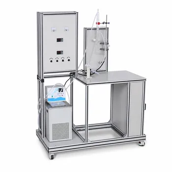
Educational pilot plants already equipped with flow visualization sections and precise flow control can be adapted by replacing the test section with a long dispersion tube. The same pumps and data acquisition systems serve the experiment, reinforcing students’ understanding of flow regime control—laminar conditions are mandatory, and any turbulence or secondary flows invalidate the measurement.

Key Calculations and Data Interpretation

From the recorded peak, students calculate the variance (σ²) of the distribution, then apply the Taylor–Aris relationship:
D = (r² * u²) / (48 * σ²)
where r is tube radius and u is average flow velocity. Plotting variance against residence time for several flow rates and verifying the linearity confirms the technique’s validity. Students then compare their resulting D values with trusted literature correlations, gaining confidence in their experimental technique.

Chromatographic Techniques: Unlocking Diffusivity from Peak Broadening

The Principle of Van Deemter and Moment Analysis

Any liquid chromatographic column exhibits band broadening due to eddy diffusion, longitudinal molecular diffusion, and resistance to mass transfer. The van Deemter equation links the height equivalent to a theoretical plate (HETP) to the mobile-phase velocity, and the molecular diffusion term directly involves D. For student laboratories, moment analysis of a single injected peak offers a straightforward route: the second central moment (peak variance) of the elution curve, corrected for extra-column effects, bears a linear relationship with 1/D under well-defined conditions.

Adapting an HPLC System for Student Measurements

A standard high-performance liquid chromatography (HPLC) system—readily available in many teaching labs—can be used without modification. Students inject a non-retained tracer (e.g., uracil for reversed-phase columns with a UV detector) at several flow rates and record the peaks. By plotting the plate height versus linear velocity and fitting the van Deemter model, the B-term coefficient yields the solute’s molecular diffusivity in the mobile phase.

This method teaches students how packed-bed hydrodynamics and stationary-phase interactions must be decoupled from pure diffusion. It also reinforces the importance of correcting for extra-column band broadening (injection volume, tubing, detector cell volume) to obtain meaningful D values.

Deriving Diffusivity from Mass Transfer Unit Operations

Using Absorption Columns and Wetted-Wall Contactors

Pilot-scale absorption towers or wetted-wall columns provide a process-centric route. Students measure the overall mass transfer coefficient (K_L a) and the specific interfacial area (a) under controlled hydrodynamics. By applying mass transfer theories—such as the penetration or surface-renewal model—that relate K_L to D, they can back-calculate the liquid-phase diffusivity. For example, in a wetted-wall column with known gas–liquid contact area, a steady-state flux measurement combined with Fick’s first law directly yields D.

Membrane Diffusion Cells: A Classic Approach

A simple side‑by‑side diffusion cell with a synthetic membrane can be integrated into a pilot plant. One chamber holds the solute solution; the other contains pure solvent. Students monitor the concentration rise in the receiver over time using conductivity or spectroscopy. By applying Fick’s second law for the appropriate geometry (slab, cylindrical, spherical) and the known membrane thickness—or by calibrating the membrane’s mass transfer resistance—they extract the diffusion coefficient. This experiment vividly connects the mathematics of unsteady-state diffusion to tangible process dynamics.

Critical Considerations for Accurate Measurements

Selecting the Right Diffusivity Model for Your System

When comparing experimental results with theoretical predictions, the choice of diffusivity correlation is paramount. The widely used Wilke–Chang model works adequately for dilute binary solutions of organic solutes, but it can exhibit errors up to 250% when water is the diffusing solute. For aqueous systems, dedicated formulations (e.g., Equation 5 of common empirical tables) reduce the average error to around 5%. Training students to select the correct model based on their chemistry prevents gross misinterpretation of mass transfer data.

The Hidden Influence of Flow Regimes on Dispersion Data

For Taylor dispersion experiments, the carrier flow must remain strictly laminar. Even minor turbulence or secondary flows caused by tube coiling, sharp bends, or pulsation destroy the premise of the derivation. Educational pilot plants that can visualize flow regimes (e.g., transparent test sections) are invaluable for demonstrating these hydrodynamic nuances. Students learn that a seemingly small irregularity can shift the measured variance and lead to a systematically underestimated diffusivity.

Understanding the Trade-offs and Common Pitfalls

No single method is universally superior. Taylor dispersion provides a direct, theory‑backed measurement with a small footprint, but it demands precise temperature control and low‑noise detectors to capture the tail of the peak accurately. Chromatographic techniques leverage existing HPLC infrastructure and are rapid, yet they require careful deconvolution of extra‑column effects and assume the solute does not interact with the stationary phase. Mass transfer unit operations (absorption, membrane cells) offer real‑world process context, but they are indirect: the result depends on assumed hydrodynamic models and interfacial area estimates, often yielding larger uncertainties.

A common mistake is neglecting temperature fluctuations; diffusivity typically changes by 1–3% per °C. Another pitfall is ignoring solvent viscosity corrections when comparing with literature values obtained under different conditions. Students must also examine the linearity of their diagnostic plots (variance vs. residence time, plate height vs. velocity) to catch systematic errors.

Making the Right Choice for Your Learning Goal

If your primary focus is measuring a reliable, fundamental diffusion coefficient with minimal modeling assumptions: Choose the Taylor dispersion method. Set up a coiled capillary with a sensitive inline detector, and validate laminar flow through pressure‑drop measurement.
If your primary focus is using existing chromatography equipment to connect separation science to transport phenomena: Perform moment analysis on an HPLC system. Start with a non‑retained tracer and carefully quantify extra‑column dispersion.
If your primary focus is demonstrating how diffusivity governs industrial mass transfer operations: Use a wetted‑wall column or a membrane diffusion cell. This lets students see the direct link between a microscopic transport property and macroscopic mass transfer rates.

Every experiment reinforces the same core principle: diffusion is not an abstract constant but a measurable, process‑controlling parameter that chemical engineers can master through thoughtful unit operations experiments.

Summary Table:

Method	Operating Principle	Key Equipment Required	Main Advantage
Taylor Dispersion	Analyzes solute band broadening in laminar flow tube	Coiled capillary tube, syringe pump, UV/RI detector	Direct, theory-backed measurement
Chromatography	Decouples diffusion from peak broadening via van Deemter	Standard HPLC system	Fast, utilizes existing lab HPLC
Mass Transfer Units	Back-calculates diffusivity from mass transfer flux	Wetted-wall column, membrane cell	Real-world industrial process context

Bring Hands-On Transport Phenomena to Your Lab

At LABPARK, we supply state-of-the-art Educational and Vocational Unit Operations Pilot Plants in chemical engineering, bioprocess & biotech, and environmental & water treatment. We empower universities, research institutes, and enterprises to bridge the gap between complex transport theory and practical engineering application.

Ready to elevate your engineering curriculum or research capabilities? Contact us today to discover how our tailored pilot plants can transform your laboratory training.