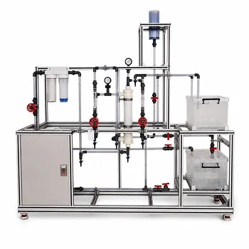
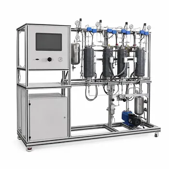
How Does The Drying Rate Change? Observe Phases On A Pilot-Scale Dryer.

The drying rate isn't constant—it evolves through three distinct phases, each governed by a different physical mechanism. In a pilot-scale convective dryer, students can directly observe this transition by tracking the material's weight loss and temperature over time, then constructing a classic drying rate curve that reveals the preheating, constant-rate, and falling-rate periods. This hands-on approach turns textbook kinetics into measurable, visual data.

A drying process is not a single event but a sequence of transport phenomena. By running a simple batch experiment on a pilot-scale tray or fluid bed dryer—holding air temperature, humidity, and velocity constant—you can plot the drying rate against moisture content. This curve is your primary diagnostic tool: it identifies the critical moisture content, shows where heat transfer controls the process and where internal diffusion takes over, and gives you the data to calculate heat and mass transfer coefficients.

The Anatomy of the Drying Rate Curve

A solid’s journey from wet to bone-dry follows a reproducible path of heat and mass transfer. Understanding each phase is essential before you can interpret what the pilot plant is telling you.

Preheating Period: The Warm-Up Stage

This is the short initial phase where the material temperature rises to the steady-state operating point. Little moisture is removed yet. The energy input primarily goes into heating the solid and bound water. In a pilot dryer, you’ll see a brief lag in weight loss while the exhaust air temperature adjusts.

Constant Rate Period: Surface Evaporation Dominance

Here, free moisture evaporates from the saturated surface as if it were an open pool of water. The drying rate stays constant because the surface remains coated with liquid, supplied fast enough by capillary action.

The rate is governed entirely by external heat and mass transfer. The material surface sits at the wet-bulb temperature of the drying air. You can calculate the drying flux using the equation $-dX/d\tau = 30(H_{as} - H)$, which links the rate directly to the humidity driving force. This means air temperature, velocity, and humidity become your direct levers. A pilot-scale dryer lets you change each of these while measuring the slope of the weight-loss curve, confirming that rate scales with the heat transfer coefficient (h) and mass transfer coefficient (K_G).

The Critical Moisture Content and the Transition

Eventually the surface can no longer remain fully wet. The moisture content at which the constant rate period ends is the critical moisture content, (X_c). This is a watershed moment. On your pilot-plant data plot of drying rate (U) vs. moisture content (X), you’ll see a sharp break in the curve. Identifying (X_c) is a primary goal of the experiment because it dictates dryer sizing and cycle design.

Falling Rate Period: Internal Diffusion Takes Over

Once the surface dries out, the drying front recedes into the solid. Internal moisture diffusion becomes the rate-limiting step. The drying rate drops continuously, and the material temperature rises toward the inlet air temperature.

In this phase, the rate often follows a linear or first-order relationship with remaining moisture, such as $-dX/d\tau = 1.2X). You can observe this on the pilot plant by plotting the derivative of your moisture-versus-time data. The falling-rate curve shape reveals internal transport properties—crucial information that cannot be guessed from theory alone, but which directly impacts total drying time at production scale.

Observing Drying Kinetics on a Pilot-Scale Dryer

A pilot-scale unit bridges the gap between a lab oven’s static dishes and an industrial operation’s dynamic environment. The goal is to generate a clean drying rate curve under constant drying conditions.

Setting Up a Constant Drying Condition Experiment

You need a convective dryer—tray dryer, fluid bed, or rotary tumble—that can hold air temperature, humidity, and velocity steady. The primary reference emphasizes pilot-scale convective dryers like fluid bed or tray units equipped with sensors. The supplementary references add that you must record initial dry weight of the solids so you can later calculate (X), the moisture content on a dry basis.

Prepare a thin, uniform bed of wet material. A thin layer minimizes internal moisture gradients during the constant-rate period, making the curve sharp and interpretable. Start the dryer, stabilize the air conditions, and then place the material inside.

Data Collection: Tracking Moisture Loss Over Time

The core measurement is weight loss. At regular time intervals, either remove and weigh the whole tray (ex-situ) or use an integrated load cell that streams live mass data.

Simultaneously, log air temperature, humidity, and—importantly—material cake temperature. During the constant-rate period, this temperature should plateau at the solvent’s boiling point under the operating pressure (or the wet-bulb temperature for water). When you see the temperature starting to rise sharply, you’ve hit the falling-rate zone. This is your independent confirmation of the critical point.

Plotting the Drying Rate Curve: From Raw Data to Insight

Take your moisture-versus-time data and convert it. First calculate the instantaneous moisture content (X) for each time point. Then use the drying rate equation (U = -\frac{G'}{S} \frac{dX}{d\tau}), where (G') is the mass of bone-dry solids and (S) is the exposed drying surface area. You can approximate the derivative by taking differences between successive time intervals.

Plot (U) on the y‑axis against (X) on the x‑axis. You will see a flat plateau (constant-rate), then a sloped decline (falling-rate). The intersection is your measured (X_c). The slope of the constant-rate plateau, combined with air conditions, lets you back-calculate the convective heat transfer coefficient (h) and the mass transfer coefficient (K_G).

Interpreting Temperature and Vapor Profiles

In a pilot unit with an agitated dryer configuration (like a rotary tumble), vapor stream composition data can supplement the curve. By tracking solvent vapor rates and cake temperatures simultaneously, students learn that the constant-rate period is a heat-transfer-controlled evaporation, while the falling-rate period becomes a mass-transfer-controlled desorption. This second view reinforces the same physics and is especially valuable when drying solvents under vacuum.

Understanding the Trade-offs and Pitfalls

The drying rate curve is a powerful tool, but misreading it—or ignoring the equipment’s side effects—can lead to flawed scale-up.

When Drying Too Fast Backfires: Defects and Case Hardening

You might think that maximizing the constant-rate period is always best. Pushing air temperature and velocity to extremes, however, can create case hardening—a dry, rigid surface layer that traps moisture inside. This artificially triggers the falling-rate period early, leaving a product that appears dry but contains high internal moisture. It also risks physical deformation, cracking, or blistering. A pilot plant lets you map the safe window of operating parameters by visually inspecting dried samples and comparing the apparent (X_c) with one obtained under gentler conditions.

Agitation Timing and Powder Quality

In agitated pilot dryers, rotating too early—when the solids are still fully saturated—can cause cohesive powders to ball up, altering bulk density and flowability. The supplementary references note that you can use the pilot plant to find the critical Loss on Drying (LOD) point where agitation should safely begin, by observing when the constant-rate period ends and the bed becomes free-flowing enough. This prevents downstream handling nightmares that scale-up would otherwise amplify.

Avoiding Entrainment and Equipment Limitations

Excessively high air velocity may fluidize or blow fine particles out of the tray. Entrainment not only corrupts your weight-loss data but also mimics a faster drying rate by mechanical removal of solids. Always confirm that your air velocity is below the entrainment threshold. The pilot plant’s transparent panels or a sight glass are your best friend here.

Making the Right Choice for Your Goal

Your specific objective will determine which aspects of the pilot-plant drying experiment you emphasize. Here’s how to focus your analysis:

If your primary focus is understanding fundamental heat and mass transfer: Concentrate on the constant-rate period. Vary one parameter at a time (air temperature, velocity, or humidity) and calculate the corresponding (h) and (K_G) coefficients from the drying flux equation. Validate against correlations.
If your primary focus is designing an industrial drying cycle: The absolute value of the critical moisture content is your most important number. Use it to determine how long you can operate in the fast constant-rate zone and when you must switch to gentler, diffusion-controlled drying to avoid defects.
If your primary focus is powder product quality: Pay attention to the transition from constant- to falling-rate as the cue for starting agitation. Then measure bulk density and particle size of the final pilot batch to ensure your drying curve doesn’t come at the cost of powder flowability.

A pilot-scale dryer does more than just dry—it gives you a window into the transport phenomena that will define your process at any scale. By mapping the full drying rate curve, you gain the kinetic fingerprint needed to predict, optimize, and troubleshoot with confidence.

Summary Table:

Drying Phase	Controlling Mechanism	Material Temperature	Pilot-Scale Observation Indicators
Preheating	Sensible heating of solid/moisture	Rises to steady-state	Lag in weight loss; adjusting exhaust air temperature.
Constant Rate	External heat & mass transfer	Plateaus at wet-bulb temp	Linear weight loss; rate changes with air velocity/temp.
Falling Rate	Internal moisture diffusion	Rises toward inlet air temp	Decelerating weight loss; material temperature spikes.

Bring Theory to Life with LABPARK Pilot Plants

Hands-on training is key to mastering drying kinetics and heat transfer. LABPARK provides state-of-the-art Educational and Vocational Unit Operations Pilot Plants in chemical engineering, bioprocess & biotech, and environmental & water treatment for universities, research institutes, and enterprises.

Equip your students and researchers with high-accuracy tools to map drying curves, identify critical moisture content, and analyze transport phenomena. Contact us today to find the perfect pilot-scale solution for your lab!