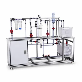
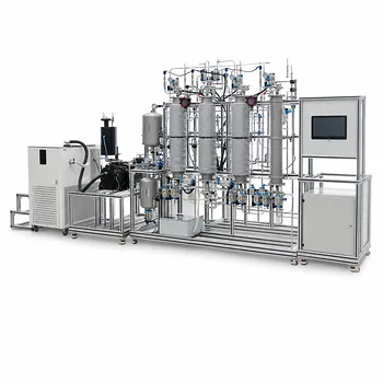
The total pressure drop is the sum of all resistance in your system, and the standard formula is ( \Delta P = 0.0001078 (\Sigma K + fL/D)\rho v^2 ). You calculate the friction factor (( f )) and the straight pipe term (( fL/D )), then simply add the resistance coefficients (( K )) for every single valve, elbow, tee, and filter before plugging values into the equation.
A pump doesn't care if resistance comes from a straight pipe or a globe valve—it just sees total energy loss. While you can correctly calculate this by summing ( K ) factors for every component, the real science of robust pilot plant design lies not just in the math, but in strategically allocating roughly 20% of that total pressure drop to your control valve to ensure stable flow regulation.
Deconstructing the Pressure Drop Components
To size a pump accurately, you must move from viewing the system as a collection of parts to viewing it as a single, unified resistance value. The pump must overcome two distinct types of loss happening simultaneously.
The Straight Pipe Loss (Major Friction)
This is the energy lost due to fluid shear along the pipe walls. It is predictable and linear relative to pipe length.
The term ( fL/D ) represents this loss. You must determine the Darcy friction factor (( f )), which depends on whether your pilot plant flow is laminar or turbulent. The total length (( L )) and internal diameter (( D )) are multiplied by ( f ), converting the physical pipe into a dimensionless resistance coefficient.
The Fitting and Valve Loss (Minor Losses)
These are actually major disruptions in a complex pilot plant. Each bend, tee, or valve core creates turbulence that dissipates energy.
The summation ( \Sigma K = K_1 + K_2 + K_3 + K_4 ) captures these losses. A standard 90° elbow might have a ( K ) factor of ( 30 f_t ), a gate valve ( 8 f_t ), and a check valve ( 50 f_t ), where ( f_t ) is the friction factor specific to the pipe size. You simply add these numbers together to create the total fitting resistance.
Two Paths to Quantifying Fitting Resistance
You don't always have access to specific ( K ) factors for exotic pilot plant components. Engineering offers two distinct methods to find this resistance, and you should know when to use each.
The Velocity Head Method (( K ) Factor)
This is the more accurate method, directly tying pressure drop to the kinetic energy of the fluid using the equation ( h = K(u^2 / 2g) ). It treats the fitting as a unique obstacle.
The method accounts for the exact geometry of the restriction. Because ( K ) factors are derived for specific flow regimes, this is the preferred approach for final equipment sizing and quantitative research.
The Equivalent Length Method (( l_e/d ))
This method is conceptually elegant: it asks, "How long would a straight pipe need to be to cause the exact same pressure drop as this valve?"
By using the ratio ( l_e/d ) (which is roughly 30 for a standard elbow), you can swap a fitting for a theoretical length of straight pipe. You can determine these values quickly using standard nomographs in the lab. This is a powerful educational tool for preliminary designs, but it is less precise because it doesn't fully capture the turbulent mixing unique to the fitting geometry.
Understanding the Trade-offs
Accurate pump sizing isn't just about getting a final number; it's about understanding where errors creep in and how the system will actually respond under dynamic control.
The Danger of Ignoring the Control Valve
If you merely sum all fixed resistances to size a pump, you will likely miss a critical design rule. A system without sufficient pressure drop across its control valve will suffer from control loop instability.
To prevent this, standard design practice mandates that the control valve consumes 15% to 25% of the total piping run pressure drop. You should include all inline devices—heat exchangers, strainers, filters—in this total run calculation. Only by allocating this "loss" can the valve operate in its optimal range and maintain a steady setpoint during your experiment.
Single-Phase vs. Two-Phase Reality
The core equation ( \Delta P = 0.0001078 (\Sigma K + fL/D)\rho v^2 ) works for a single, incompressible liquid. If your pilot plant has a gas-liquid mixture (two-phase flow), the logic changes.
In two-phase flow, you can still use proportionality. First, calculate a baseline pressure loss for a standard 90-degree elbow using the phase flow rates and densities. Then, multiply that value by specific geometry multipliers (e.g., 2.5 for a check valve, 3.0 for an angled tee). Summing these proportional losses accounts for the unique acceleration effects mixed phases have in fittings. For elevation changes, you must use a correction factor like the Flanigan method rather than a simple density-based static head.
Making the Right Choice for Your Goal
While the methodology is universal, your approach to calculation fidelity should match the objective of your pilot plant.
- If your primary focus is research accuracy: Use the velocity head method with specific ( K ) factors for every component and strictly validate the friction factor for your flow regime. The accuracy of your pump curve match depends on this precision.
- If your primary focus is educational design efficiency: Use the equivalent length method with nomographs to speed up early design iterations. This simplifies the visualization of total system resistance for students.
- If your primary focus is safe, stable operation: Start your design by subtracting 20% of the available pump head for the control valve, then solve the pressure drop equation for the remaining piping and fittings. A pump sized without this allocation will almost certainly result in poor flow control.
By treating the piping system as an algebraic sum of resistances and a strategic allocation of pressure for the control device, you can confidently specify a pump that delivers the right flow and stable automation.
Summary Table:
| Loss Type | Key Equation / Method | Primary Cause | Design Focus |
|---|---|---|---|
| Major Loss | Darcy Friction Factor ($fL/D$) | Fluid shear along pipe walls | Pipe length and diameter |
| Minor Loss | Velocity Head ($K$ Factor) or Equivalent Length ($l_e/d$) | Turbulence in valves and fittings | Geometry of restrictions |
| Control Valve Loss | 15% to 25% of total piping run drop | Dynamic control regulation | Loop stability |
Optimize Your Pilot Plant Design with LABPARK
Designing efficient piping systems and sizing pumps accurately requires specialized engineering expertise. LABPARK provides state-of-the-art Educational and Vocational Unit Operations Pilot Plants in chemical engineering, bioprocess & biotech, and environmental & water treatment.
Whether you represent a university, research institute, or enterprise, we deliver robust, high-performance systems engineered for precise flow control, stable automation, and reliable scale-up. Let our technical experts help you customize the perfect system for your lab.
Contact LABPARK Today to discuss your project requirements and request a quote!
Related Products
- Multi Pump Fluid Transport Process Piping Unit Operations Training Pilot Plant
- Fluid Transport and Piping Dynamics Practical Training Unit Operations Pilot Plant
- Chemical Pipeline Assembly and Fluid Transport Practical Training Unit Operations Pilot Plant
- Hollow Fiber Ultrafiltration Membrane Separation Educational Pilot Plant
- 100L Continuous Loop Hydrogenation Educational Unit Operations Pilot Plant
People Also Ask
- Why distinguish Newtonian & non-Newtonian fluids in pilot plants? Prevent design errors.
- How do steady-state and dynamic simulations complement pilot plants? Validate scale-up and controllability
- How can unit operations pilot plants demonstrate simultaneous removal of light and heavy impurities? Configure a modular setup
- How can chemical engineering students use unit operations pilot plants to study kinetics? Master reactor scale-up!
- Why is the chemical plant startup schedule crucial? De-risk scale-up with pilot plants.