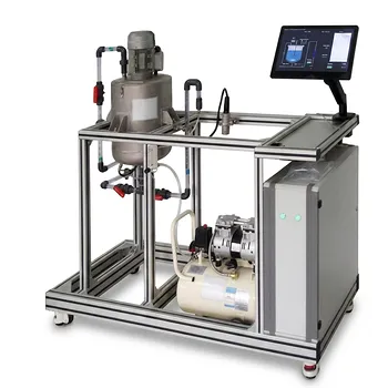
How Do Fluid Mechanics Units Demonstrate Pitot Tube Differences? Master Open Vs. Closed Flow Setups.

The difference hinges on the role of static pressure. Fluid mechanics training units demonstrate this by contrasting two scenarios. In an open stream, a single tube facing upstream is enough because the liquid’s rise above the free surface directly equals the velocity head. In a closed, pressurized conduit, you must measure both the stagnation pressure and the static pressure outside the tube—the differential between them yields the velocity head. The training unit makes this abstract principle tangible by letting you see and measure the fluid columns in each case.

The core takeaway is that an open-stream Pitot tube uses the surrounding free surface as its static pressure reference, while a closed-conduit measurement requires a separate static pressure tap. The unit proves that velocity in both cases comes from the same fundamental equation, but the measurement configuration must adapt to whether the flow is bounded and pressurized.

The Foundational Principle: From Stagnation to Velocity

A Pitot tube works by converting kinetic energy into potential energy in the form of pressure. Fluid mechanics training units are built around the stagnation pressure equation:

$p_2 = p_o + \rho V_o^2 / 2$

Here, $p_2$ is the stagnation pressure measured at the tube’s opening, $p_o$ is the local static pressure, and the last term is the dynamic pressure. The unit physically shows this energy balance by allowing fluid to rise in a manometer column.

Visualizing the Equation in an Open Stream

The training unit’s open channel or free jet setup isolates the simplest case.

The free surface provides a zero-velocity-head reference. In an open stream, the surrounding liquid surface is at atmospheric pressure. When you insert a Pitot tube facing upstream, the fluid rises in the tube above that surface. The instructor points out that this height difference is exactly the velocity head $V^2/(2g)$.

The unit makes it clear that no second measurement is needed. The static pressure is already known—it’s the pressure at the free surface. Students can directly read the local stream velocity from a single manometer tube.

Adapting to a Pressurized Conduit

When the training unit shifts to a closed, pressurized pipe, the demonstration changes fundamentally.

The static pressure is no longer atmospheric. Inside a pipe, the fluid is under pressure from the system. So, $p_o$ in the equation is an unknown value, often much higher than atmospheric.

To solve for velocity, the unit introduces a second measurement point—a static pressure tap in the pipe wall or on a combined Pitot-static tube. One manometer leg goes to the stagnation port, the other to the static port. The differential height between the two columns gives the dynamic pressure directly, subtracting the static pressure that would otherwise obscure the velocity reading. Without this, you’d be measuring total pressure only and have no way to separate the kinetic contribution.

Beyond the Demonstration: Getting a Read You Can Trust

Training units don’t stop at the two-case principle; they also embed the real-world conditions needed for a believable measurement.

Placement: The Fully Developed Flow Mandate

The supplementary references stress that the unit must place the Pitot tube in a stable, fully developed flow region.

Any upstream disturbance—a valve, an elbow, or a change in pipe diameter—distorts the velocity profile. The training rig typically includes a long, straight run of piping before the measurement station to let the flow settle. This is not just a theoretical nicety; it’s built into the unit’s plumbing to prevent students from seeing erratic, unrepresentative readings.

Sizing and Alignment: The Probe as a Ghost

The physical probe itself can disrupt the very velocity it tries to measure. The training unit models the critical rule: the probe’s outer diameter must be less than 1/50 of the pipe’s inner diameter.

A probe tip that is too large blocks the flow, creating a false, elevated pressure reading. The demonstration also enforces perfect alignment. The opening must point directly into the flow—parallel to and against the fluid direction—or the reading will be low. Many units use clear pipe sections to let observers see the wake and verify the probe’s position.

From Local Point to Average Flow

A Pitot tube measures velocity at a single point. The training unit typically places it at the centerline, where velocity is highest ($u_{max}$).

But most engineering applications need the average velocity ($u$) to calculate flow rate. The instructor uses a chart or reference that relates the ratio $u/u_{max}$ to the Reynolds number. Students perform the calculation, and the unit often integrates a flow meter to validate the converted average. They learn that the final step is applying a calibration coefficient (C, typically 0.98–1.00) to compensate for slight manufacturing variations in the probe’s geometry.

Understanding the Trade-offs and Common Pitfalls

No measurement technique is flawless. The training unit clarifies these limitations so users don’t take the numbers at face value.

The Pitot tube gives a local velocity, not the whole picture. If you need the total flow rate, you must either traverse the probe across the pipe’s diameter or rely on the $u/u_{max}$ relationship, which is only accurate for well-known turbulent profiles.

It is sensitive to installation errors. A tiny angle misalignment or insertion too close to a disturbance can introduce errors larger than 5–10%. The clear-pipe demonstration often shows how a slight tilt dramatically reduces the manometer reading.

The probe is intrusive, even when properly sized. In very small pipes or viscous flows, the diameter rule (D/50) can still cause blockages. This can increase the upstream pressure, giving a falsely high velocity. The unit’s manometer might appear stable, but the number would be wrong.

Calibration is not optional. The textbooks might give a coefficient of 0.98, but the unit’s actual probe might differ slightly if it’s been nicked or not perfectly machined. You must verify or at least be aware that the reading is only as accurate as the calibration constant you use.

How to Apply This to Your Own Lab or Project

Whether you’re setting up a training unit or just interpreting a single velocity reading, your approach should match your goal.

If your primary focus is teaching the fundamental difference between open and closed systems: Use a unit with a convertible setup—one that can run as an open jet and then switch to a closed loop. Point out that the open case uses just one manometer tube while the closed case requires a differential manometer across stagnation and static ports.
If your primary focus is ensuring accurate measurements in a closed conduit: Prioritize probe sizing (under D/50), install it far downstream of any disturbances, and verify alignment visually if possible. Always take the centerline reading first and then decide if you need a complete traverse or a Reynolds-number correction to get the average velocity.
If your primary focus is demonstrating error sources to new engineers: Deliberately misalign the probe, insert it too close to a bend, or use an oversized probe. Show how the manometer reading changes. Then correct the setup and compare the values—this builds an intuitive distrust of raw numbers that is priceless in industry.

Understanding the two faces of the Pitot tube—open stream versus pressurized conduit—is about grasping where your static pressure reference comes from. Once that principle is clear, the training unit’s manometer will always tell you an honest story.

Summary Table:

Feature	Open Stream	Closed Pressurized Conduit
Static Pressure Reference	Atmospheric (uses free surface)	System-dependent (requires wall/static tap)
Manometer Configuration	Single tube facing upstream	Differential manometer (stagnation + static ports)
Velocity Head Calculation	Directly equals fluid rise height	Equals differential height between ports
Critical Setup Factor	Free surface stability & alignment	Probe size ($< D/50$) & flow profile (Reynolds No.)

Bring Fluid Dynamics to Life in Your Lab

Teaching fluid mechanics requires hands-on, high-precision equipment that bridges theory and practice. LABPARK provides state-of-the-art Educational and Vocational Unit Operations Pilot Plants in chemical engineering, bioprocess & biotech, and environmental & water treatment.

Designed specifically for universities, research institutes, and enterprises, our advanced training rigs make complex concepts like Pitot tube measurements, flow dynamics, and pressure drops visually clear and highly tangible for students and researchers alike.

Ready to upgrade your laboratory training systems? Contact us today to discuss your custom pilot plant requirements and receive a tailored solution!