How Do Pilot Plants Utilize Ion-Interaction Vs. Association Models? High-Salinity Simulation Guide.

The moment you begin modeling a high-salinity stream, you face a fork in the road. Chemical engineering and water treatment pilot plants leverage the thermodynamic gulf between ion-interaction and ion-association models to directly compute phase equilibria or to iteratively resolve speciation. They use the ion‑interaction framework for efficient, single‑step Gibbs‑energy calculations that predict scaling, osmotic pressure, and bulk phase behavior in multicomponent brines. For systems dominated by discrete ion pairs—especially transition metals—they switch to the ion‑association model, but never blend the two, because mixing their independent parameter sets leads to fatal thermodynamic errors.

The ion‑interaction model delivers direct Gibbs energy of the aqueous phase for rapid phase‑equilibria predictions, while the ion‑association model requires iterative speciation calculations suited for specific ion‑pair‑dominated systems. Pilot plants exploit this difference by choosing the pathway that matches the simulation goal and rigorously avoiding any cross‑pollination of parameters.

The Thermodynamic Divide Between Two Modeling Philosophies

Direct Gibbs Energy vs. Iterative Speciation

The ion‑interaction model (e.g., the Pitzer framework) expresses the excess Gibbs energy of the entire aqueous solution through empirical binary and ternary parameters. It gives you activity coefficients and chemical potentials in a single, non‑iterative step, making it exceptionally efficient for predicting vapor‑liquid, solid‑liquid, and liquid‑liquid equilibria in concentrated electrolytes like seawater or brine concentrates.

The ion‑association model assumes that genuine ion pairs or complexes form in solution. It requires solving a system of equilibrium formation constants to determine the true species distribution (speciation) before any bulk thermodynamic property can be calculated. That nested iteration is slower but captures the chemistry of systems where strong, specific complexes—like those of transition metals—dominate behavior.

How Pilot Plants Exploit the Computational Difference

In a pilot‑plant control room, decisions must be fast. Simulating feed‑side osmotic pressures for a reverse‑osmosis unit or predicting the supersaturation index of gypsum across a temperature range needs direct, analytically robust outputs. The ion‑interaction model delivers those without an inner speciation loop, fitting seamlessly into dynamic process simulators.

Conversely, when a pilot handles industrial wastewater laden with copper, zinc, or heavy‑metal complexes, the speciation from an ion‑association model reveals whether soluble hydroxo‑complexes or solid precipitates will form. This targeted, slower calculation is reserved for the trace‑level challenge, not for the bulk matrix.

Why Mixing Models Leads to Catastrophic Errors

Independent Thermodynamic Assumptions Cannot Merge

Ion‑interaction parameters are regressed from experimental data under the assumption that no discrete ion pairs exist; they are “effective” pairwise energies. Ion‑association equilibrium constants, on the other hand, are measured under the assumption that the free‑ion activities are the driving force for explicit complex formation. Pulling a Pitzer parameter into a law‑of‑mass‑action speciation equation—or vice versa—double‑counts interactions and violates the law of mass action. The result is a thermodynamic chimera that produces nonsensical saturation indices, erroneous pH shifts, and wildly inaccurate chemical‑dosing forecasts.

The Practical Fallout in a Pilot Plant

An operator who mixes ion‑interaction activity coefficients with ion‑association stability constants could misinterpret the scaling risk of calcium carbonate or completely mis‑predict when a trace metal will precipitate. In a membrane pilot, that might lead to severe fouling within hours. In a thermal brine concentrator, mixed‑model errors can hide the true boiling‑point elevation, causing poor heat‑transfer design. Pilot plants therefore treat the two models as separate toolboxes, never opening both on the same simulation canvas without a rigorous, research‑grade reconciliation protocol.

Applying the Right Model in Pilot-Plant Operations

Targeted Use for Separation Processes

For thermal desalination or multi‑stage flash pilots, the ion‑interaction model directly gives boiling‑point elevation and the solubility limits of common scalants (CaCO₃, CaSO₄, Mg(OH)₂). The operator can tune antiscalant doses against reliable supersaturation ratios without waiting for iterative calculations.

For industrial wastewater pilots rich in nickel or chromium, the ion‑association model predicts which pH range keeps these metals dissolved as neutral or anionic complexes, guiding the ion‑exchange or chemical precipitation step.

Validating the Chosen Model with Analytical Measurements

Pilot plants often bridge the theoretical gap with bench‑scale checks. For example, a simple cation‑exchange column—eluting with acid and titrating the effluent—can measure total cation equivalents and hydroxide/carbonate alkalinity splits. That experimental value can be compared directly against the model’s predicted speciation to see whether the ion‑association framework actually reflects reality, or whether an ion‑interaction approach would have sufficed for the bulk water chemistry.

Guarding Membrane‑Scaling Predictions

When a reverse‑osmosis pilot processes a high‑salinity feed, the scaling potential of sparingly soluble salts must be known with high confidence. An ion‑interaction model provides traceable activity coefficients for all major ions in one consistent framework. If the feed also contains a problematic transition metal, a separate, offline ion‑association simulation determines the metal’s solubility limit, but those results are not fused into the bulk model. The operator maintains a firewall between the two thermodynamic descriptions to preserve accuracy.

Understanding the Trade‑offs

Ion‑Interaction Strengths and Blind Spots

The ion‑interaction model is fast, robust, and parameter‑rich for many common electrolyte systems. It handles high ionic strengths gracefully. However, it treats all ions as fully dissociated and fails to represent strong, specific complexes unless those are implicitly absorbed into the empirical parameters—a fragile approximation when the complexation chemistry changes with redox conditions or ligand additions.

Ion‑Association Precision and Bottlenecks

Ion‑association models shine at predicting trace‑metal speciation and redox‑sensitive complexes. Their Achilles’ heel in high‑salinity waters is the scarcity of reliable stability constants at extreme ionic strengths, where activity‑coefficient corrections to the free‑ion model become heavily uncertain. The iterative solution also demands more computational time, which can be a drawback in real‑time process control.

The Non‑Negotiable Cost of Mixing

The gravest trade‑off appears when someone tries to combine the two—tempted by the desire to capture both bulk colligative properties and specific complexation in a single pass. The thermodynamic inconsistency outweighs any perceived benefit, producing predictions that are worse than either model alone. Consequently, the most valuable practice in a pilot plant is to maintain a clear boundary: model the bulk matrix with ion‑interaction, model the trace actors with ion‑association, and only compare outputs, never merge parameters.

Making the Right Choice for Your System

Select your thermodynamic pathway based on what you need to predict and the nature of the aqueous system under test.

If your primary focus is bulk phase equilibria (scaling, boiling‑point elevation, osmotic pressure) in a multicomponent brine: Stay within a pure ion‑interaction framework like Pitzer. You gain speed, consistency, and reliable saturation indices for major scalants.
If your focus is on trace‑metal behavior or specific ion‑pair‑driven chemistry (e.g., heavy‑metal solubility, hydrolysis complexes): Invest in an ion‑association model with carefully curated stability constants, but run it separately. Do not attempt to blend its constants with the bulk model’s activity coefficients.
If you are integrating a membrane process simulation in real time: Use ion‑interaction for the continuous phase‑equilibria loop. Validate the results against independent, offline ion‑association calculations for any critical trace species that could compromise the membrane.

By keeping the two thermodynamic worlds separate, pilot‑plant engineers turn a confusing model jungle into a clear divide‑and‑conquer strategy—one that safeguards process predictions from the very first bench test to full‑scale installation.

Summary Table:

Feature	Ion-Interaction Model	Ion-Association Model
Primary Focus	Bulk phase equilibria & activity	Discrete ion pairs & chemical speciation
Calculation Method	Direct, non-iterative Gibbs energy	Iterative solving of equilibrium constants
High-Salinity Performance	Excellent (robust empirical parameters)	Limited by uncertainty at extreme ionic strength
Key Application	Desalination, RO, boiling-point elevation	Heavy metal precipitation, toxic wastewater

Optimize Your Chemical Engineering & Water Treatment Processes

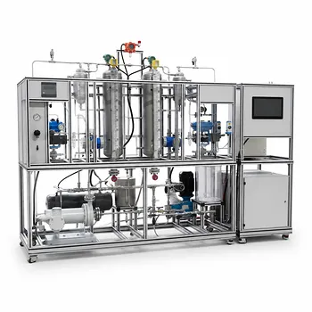
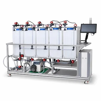
Transitioning from thermodynamic models to physical validation requires precise, reliable equipment. LABPARK provides premium Educational and Vocational Unit Operations Pilot Plants in chemical engineering, bioprocess & biotech, and environmental & water treatment. Designed specifically for universities, research institutes, and enterprises, our systems enable you to validate scaling, filtration, and phase equilibria models under real-world conditions.

Ready to elevate your research and training capabilities? Contact LABPARK today to discuss your custom pilot plant requirements!