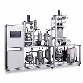
How Can The Distribution Coefficient (Kd) Be Calculated? Optimize Extraction Pilot Plant Experiments.

Calculating the distribution coefficient (KD) is the bedrock of any meaningful countercurrent extraction experiment. In a pilot plant setting, you can determine KD directly from actual operating data using the end-stream compositions—specifically, the solute loading in the entering solvent and the exiting raffinate. For dilute systems, you can estimate KD from Henry’s law constants and molecular weights. Both approaches empower you to rate column performance, quantify mass transfer efficiency, and scale processes with confidence.

KD captures the solute’s thermodynamic preference for the solvent over the feed, and experimental KD values translate pilot-plant data into actionable design criteria. Whether derived from measured stream compositions or predicted from gas solubility data, the coefficient is the linchpin for identifying inefficiencies and sizing industrial columns.

What the Distribution Coefficient Represents in Extraction

The Physical Meaning of KD

KD is the ratio of solute concentration in the extract phase to that in the raffinate phase at equilibrium. On a practical, mass‑ratio basis, it defines how many parts of solute go into the solvent for every part remaining in the feed. This single number dictates the required solvent‑to‑feed ratio and the number of stages needed for a given separation.

Why KD is Central to Pilot‑Plant Experiments

In a countercurrent pilot column, real‑world non‑idealities—axial mixing, entrainment, variable mass transfer rates—blur the ideal equilibrium picture. Measuring an effective KD from operating data bridges the gap between textbook thermodynamics and actual plant behavior. It lets you quantify how close your column comes to ideal staging, diagnose bottlenecks, and generate reliable scale‑up parameters.

Calculating KD Directly from Operating Data

The End‑Stream Composition Method

The primary route for a running pilot plant uses the compositions of the two streams that interact at one end of the column. At steady state, KD = [Se₁ / (1 + Se₁)] / [We₁ / (1 + We₁)].

Se₁ is the mass of solute per unit mass of entering solvent (on a solute‑free basis).
We₁ is the mass of solute per unit mass of exiting raffinate (also solute‑free).

The fractions Se₁/(1+Se₁) and We₁/(1+We₁) convert these mass ratios into weight fractions, giving a dimensionless KD that directly reflects the solute partitioning at that column end.

Practical Steps in the Lab

Sample stream pairs simultaneously at the end where fresh solvent meets the spent raffinate.
Perform a mass balance to confirm steady‑state operation (inlet feed solute ≈ outlet raffinate solute + outlet extract solute).
Analyze each sample to obtain the solute mass per mass of pure solvent or pure diluent.
Plug the numbers into the formula. The result is the effective KD for that end stage, which can be compared to equilibrium values to assess stage efficiency.

Interpreting the Result

When the column stage is perfectly efficient, the calculated KD equals the thermodynamic equilibrium value. A lower experimental KD indicates mass transfer limitations—the exiting raffinate carries more solute than equilibrium would predict. Repeating the measurement at both ends and at several operating conditions reveals how efficiency varies with throughput.

Estimating KD for Dilute Systems Using Henry’s Law

The Thermodynamic Shortcut

For systems where solute concentrations stay below about 20% by weight, you can bypass extensive pilot measurements. KD can be estimated from the solute’s Henry’s law constants in the two liquid phases:
KD = (Hf / Hs) × (MWs / MWf)

Hf = Henry’s constant of the solute in the feed liquid.
Hs = Henry’s constant of the solute in the solvent liquid.
MWs, MWf = molecular weights of the solvent and feed (solute‑free basis).

This relation converts gas‑liquid Henry’s constants into a liquid‑liquid distribution ratio, assuming ideal, dilute behavior.

Leveraging Existing Gas Solubility Data

Because Henry’s constants are widely tabulated, you can quickly screen solvents without running a single experiment. Chemical engineering laboratory courses often use this approach to teach students how to predict extraction performance from databases, dramatically shortening the learning cycle.

Where the Henry’s Law Method Fits

It excels in early‑stage feasibility studies, when pilot‑plant data is not yet available, or when the solute‑solvent system is known to be dilute and moderately non‑ideal. Never extrapolate it to concentrated systems without verifying against actual equilibrium data—deviations grow quickly as solute‑solute interactions become significant.

Applying KD Values in Pilot‑Plant Experiments

Rating Extraction Column Performance

Once you have an experimental KD, combine it with the operating line and material balance to calculate the number of theoretical stages or the height equivalent to a theoretical plate (HETP). Comparing the measured HETP to manufacturer‑supplied benchmarks tells you if packing is fouled, channeling is occurring, or the column is simply undersized.

Scaling Up with Confidence

Scale‑up from a pilot column relies on the same KD. If the effective KD remains constant with scale, you can use pilot‑derived HETP values to design a full‑size column that achieves the same separation. The formula from operating data also reveals whether a different solvent‑to‑feed ratio could improve throughput without sacrificing purity.

Diagnosing Mass Transfer Efficiency

A persistent gap between the thermodynamic KD (from equilibrium measurements) and the field KD (from the end‑stream method) is a red flag. It signals poor phase dispersion, low interfacial area, or back‑mixing. Addressing these factors often yields a bigger capacity gain than simply adding column height.

Understanding the Limitations and Pitfalls

The End‑Stage Equilibrium Assumption

The primary formula presumes that the two streams at the sampled end are in equilibrium. In a real column, that stage rarely achieves 100% efficiency. The computed KD is therefore an apparent value, not a true thermodynamic constant. Always validate it by measuring actual equilibrium in a shake‑flask test for the same composition.

Concentration‑Dependent Behavior

KD is rarely a single number across the whole column. If solute partitioning is nonlinear, the value measured at the lean end may differ from the value at the rich end. For accurate column modeling, you need a KD profile, not just one point.

Limits of the Henry’s Law Approximation

The gas‑solubility method relies on dilute‑solution ideality. Above about 20 weight percent solute, activity coefficients deviate significantly, and the predicted KD can be off by a factor of two or more. Always corroborate with experimental points before committing to a column design.

Making the Right Choice for Your Goal

Different stages of a project demand different levels of accuracy and effort. Use this guide to align your method with your objective:

If your primary focus is rating an existing pilot column or generating scale‑up parameters: Rely on the end‑stream composition method. It captures real‑plant non‑idealities and gives you the effective KD needed for HETP and stage calculations.
If your primary goal is early‑stage solvent screening or teaching fundamental concepts: Use the Henry’s law estimation. It allows rapid comparisons without pilot‑plant runs and teaches students how to translate gas‑solubility data into extraction design.
If your system is concentrated or highly non‑ideal: Perform equilibrium measurements across the full concentration range and refine your KD values with activity‑coefficient models; the simple operating‑data formula will only give an apparent snapshot, not a design‑ready parameter.
If you need to troubleshoot mass transfer inefficiencies: Calculate KD from both end stages, compare them, and benchmark against thermodynamic equilibrium. A mismatch points directly to hydrodynamics or packing issues that require attention.

With a clear KD in hand—whether measured at the pilot column or predicted from first principles—you transform a routine unit‑operations experiment into a robust foundation for industrial extraction design.

Summary Table:

Method	Key Formula / Basis	Best Use Case	Main Limitation
End-Stream Composition	$K_D = \frac{Se_1/(1+Se_1)}{We_1/(1+We_1)}$	Rating existing pilot columns & process scale-up	Yields apparent, not true thermodynamic, $K_D$
Henry's Law Estimation	$K_D = (\frac{H_f}{H_s}) \times (\frac{MW_s}{MW_f})$	Early solvent screening & academic instruction	Limited to dilute systems ($<20%$ solute)

Bring Industrial Reality to Your Laboratory

Are you looking to bridge the gap between academic theory and industrial scale-up? LABPARK provides high-quality Educational and Vocational Unit Operations Pilot Plants in chemical engineering, bioprocess & biotech, and environmental & water treatment. Designed specifically for universities, research institutes, and enterprises, our pilot plants enable students and researchers to perform precise countercurrent extraction experiments, calculate exact thermodynamic parameters, and scale up chemical processes with confidence.

Ready to upgrade your lab's capabilities? Contact LABPARK today to discover how our custom pilot plant solutions can enhance your research and teaching efficiency.