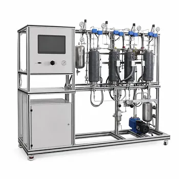
How Can Chemical Engineering Students Use A Drying Unit Operations Pilot Plant To Experimentally Determine The Drying Rate Curve And Critical Moisture Content Of A Solid Material?

The definitive method for experimentally determining a drying rate curve begins with precise gravimetric data. In a pilot-scale tray or convective dryer, students maintain constant air temperature, humidity, and velocity while continuously recording the time and the corresponding weight of the wet solid. By converting this raw weight-loss data into moisture content (dry basis) and applying the fundamental rate equation $U = -\frac{G'}{S} \frac{dX}{d\tau}$, you can generate the classic drying rate curve to pinpoint exactly where the constant-rate period ends and the falling-rate period begins.

Understanding the transition between the constant and falling-rate periods is the core challenge. The critical moisture content ($X_c$) is not a universal material constant; it is an experimentally determined inflection point on the drying rate curve where the surface can no longer stay saturated, causing the drying mechanism to shift from external heat-transfer control to internal mass-transfer control.

Executing the Pilot Plant Experiment

The Core Gravimetric Technique

The foundation of this experiment relies on tracking mass loss over time. Since the primary goal is to calculate $U$ (drying rate), you must generate a smooth curve of moisture content ($X$) versus time ($\tau$).

In a tray dryer pilot plant, this typically involves removing a tray at specific intervals to weigh it on an external balance. While straightforward, this method introduces manual interruption. For a more precise data set, a convection pilot unit equipped with a built-in load cell allows for non-invasive, continuous data logging. This captures real-time $X$ values, making it easier to numerically differentiate the data to find the critical point.

Calculating and Plotting the Drying Rate

Raw time-weight data is not yet a rate curve. You must convert it using the drying area ($S$) and the bone-dry mass ($G'$).

Determining the bone-dry mass ($G'$) is a critical step that must happen after the experiment concludes. You dry the solid in an oven at a higher temperature until there is no further weight loss, ensuring all free and bound moisture is removed. Once $G'$ is known, you calculate the moisture content for every previous data point as $X = \frac{\text{mass of water}}{\text{mass of bone dry solid}}$. The drying rate is then derived by analyzing the slope of the $X$ vs. $\tau$ curve, scaled by the constant ratio $\frac{G'}{S}$. Plotting this calculated rate ($U$) against the free moisture content ($X$) reveals the distinct drying phases.

Interpreting the Curve and Critical Point

The Constant-Rate Period Physics

At the start of the curve, you will observe a horizontal line. This is the constant-rate period, where the solid surface behaves like a pool of free water.

During this phase, the controlling resistance is external heat transfer. The rate of evaporation is governed purely by how fast heat from the hot airstream can be transferred to the wet surface. The material temperature validates this theory. By inserting a thermocouple just below the surface, students should observe that the solid's temperature stabilizes precisely at the air's wet-bulb temperature, remaining constant throughout this phase.

Identifying the Critical Moisture Content ($X_c$)

The critical moisture content ($X_c$) is the point where the horizontal line begins to curve downward. It marks the moment the internal physics of drying fundamentally change.

This transition occurs because internal capillary forces can no longer pump moisture to the surface fast enough. The surface starts to develop dry patches, and the drying rate begins to drop as the "wet front" recedes into the solid. You will observe a corresponding rise in material temperature at this exact transition point. When the surface dries out, evaporative cooling slows, and the solid temperature begins a steady climb toward the dry-bulb temperature of the incoming air.

The Falling-Rate Period Analysis

After $X_c$, the curve is dominated by internal mass transfer. This segment is often non-linear, highlighting the complex diffusion mechanisms within the solid's pores.

The falling-rate zone is where drying becomes energy-intensive and slow. Removing small amounts of residual moisture takes a disproportionate amount of time. The shape of this falling-rate curve is crucial for scale-up, as it allows you to model the relationship between the declining drying rate and the residual moisture, which is necessary to accurately predict total residence time in an industrial dryer.

Understanding the Trade-offs

Limitations of Pilot Plant Data

While pilot plants provide essential design data, certain pitfalls can skew the results or limit their applicability to commercial-scale units.

A "constant" drying condition is an idealization. In a real pilot plant, even small fluctuations in air velocity or inlet humidity can introduce noise into your weight-loss data, making it difficult to accurately calculate the derivative ($dX/d\tau$) right at the inflection point. The determined $X_c$ is highly specific to bed depth. A tray experiment using a 2 cm deep bed will yield a completely different critical moisture content than a 5 cm deep bed, because the mass transfer path length changes. Students must strictly control and report sample thickness, as this value cannot be generalized. Static tray data does not scale to agitated dryers. If you are designing a fluid-bed or paddle dryer, a static tray pilot unit will overestimate drying time because mechanical agitation continuously exposes new wet surfaces, fundamentally altering the falling-rate mechanism.

Applying This to Your Design Project

The choice of how you process and use this experimental data depends entirely on your engineering objective.

If your primary focus is scaling up a convective dryer: Use the constant-rate data to calculate the heat transfer coefficient ($h$) and mass transfer coefficient ($K_G$). These values are the core scaling parameters that will allow you to size the full-scale unit.
If your primary focus is minimizing energy consumption: Analyze the slope of the falling-rate curve. Optimizing when to stop the drying cycle—rather than extending the time to chase a tiny fraction of residual moisture—will yield the largest savings in thermal energy.
If your primary focus is protecting a heat-sensitive product: Pay close attention to the temperature trace near the critical point. You must design the process so the product exits the dryer shortly after $X_c$ is reached, preventing exposure to the rising temperatures of the late falling-rate period.

Mastering this specific experimental method transforms the drying curve from an abstract textbook concept into a practical diagnostic tool, allowing you to directly see where a process shifts from efficient surface evaporation to the costly, diffusion-limited zone.

Summary Table:

Feature / Parameter	Constant-Rate Period	Falling-Rate Period
Controlling Resistance	External heat & mass transfer	Internal mass transfer (diffusion)
Solid Surface State	Fully saturated (constant wetness)	Dry patches / receding wet front
Material Temperature	Constant (at wet-bulb temperature)	Rising (approaching dry-bulb temp)
Drying Rate ($U$)	Constant (horizontal line)	Declining (non-linear curve)

Elevate Your Chemical Engineering Lab with LABPARK

Bridge the gap between textbook theory and practical application. LABPARK provides premium Educational and Vocational Unit Operations Pilot Plants in chemical engineering, bioprocess & biotech, and environmental & water treatment for universities, research institutes, and enterprises.

Our drying pilot plants feature integrated data logging and precise control systems, enabling students and researchers to capture accurate gravimetric data and master drying kinetics.

Contact LABPARK today to discover how our pilot plants can enhance your department's hands-on training and research capabilities!