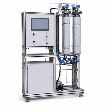
Suspended particles are the silent saboteurs of online UV-vis spectroscopy in wastewater pilot plants. They scatter light, creating a turbidity-based baseline shift across the absorption spectrum. This shift directly violates the linear relationship described by Beer’s Law, causing the instrument to report erroneously high or unstable concentrations. To resolve this, you either apply a simple baseline correction using a non-absorbing reference wavelength, or, when scattering produces a complex, sloping baseline, you deploy multivariate chemometric techniques like partial least squares (PLS) or derivative filtering to mathematically isolate the true analyte signal from particle interference.
Suspended solids introduce light scattering that manifests as a broad baseline elevation or slope in a UV-vis spectrum, destroying the direct proportionality between absorbance and concentration. Resolving it means choosing between a rapid, single-wavelength subtraction method for stable, flat offsets and a more sophisticated chemometric model that decouples scattering from absorption in complex, variable samples. The right choice depends entirely on your wastewater’s particle load and your pilot plant’s need for real-time accuracy versus modeling effort.
The Physics of the Problem: How Particles Distort UV-Vis Spectra
Scattering and the Birth of the Baseline Shift
In a perfectly clear solution, light passes straight through the sample. When suspended particles are present, photons collide with these particles and are deflected in all directions. The detector sees a loss of transmitted light that is not from absorption but from scattering.
This lost light registers as an apparent absorbance. Because scattering is not strongly wavelength-specific, it appears as a broad, featureless elevation across the entire spectrum. This is the turbidity baseline shift. In practice, smaller particles can also cause a wavelength-dependent slope, where scattering becomes more intense at shorter wavelengths, creating a tilted baseline rather than a flat one.
Why This Breaks Beer’s Law in Pilot Plants
Beer’s Law ($A_{\lambda} = \varepsilon_{\lambda} b C$) demands that absorbance at a specific wavelength stems purely from the target chemical species. The baseline shift adds an unknown, time-varying offset to that absorbance. The result is a combined signal: true absorption plus a scattering artifact.
In an online pilot plant, this means your real-time concentration readings for TOC, DOC, or specific pollutants become inflated and noisy. A control system relying on this data will trigger unnecessary dosing or misdiagnose treatment failure, undermining the very purpose of continuous monitoring.
Resolving Particle Interference: From Simple Subtraction to Advanced Chemometrics
Baseline Correction for Flat Shifts
When the baseline offset is constant across the spectrum, the fix is straightforward. You select a reference wavelength where your analyte does not absorb but where the scattering signal remains. By subtracting the absorbance at this reference wavelength from the absorbance at your analytical wavelength, you mathematically remove the scattering offset.
This is the classic two-wavelength correction. It works well in many secondary treatment effluents where particle size distribution is relatively stable and the baseline is genuinely flat. It is computationally simple, transparent, and easy to validate.
Derivative Techniques for Sloping Baselines
A flat reference subtraction fails when the scattering baseline is sloped—a common scenario with fine colloids that scatter more light in the UV. First- and second-derivative spectroscopy can filter out this constant or linear baseline.
By calculating the derivative of the spectrum, you amplify narrow absorption bands and suppress the broad, slowly varying scattering signal. A first derivative removes a constant offset; a second derivative removes a linear slope. This approach requires no chemometric model but does amplify noise and can make spectra harder to interpret visually.
Multivariate Chemometric Models
For pilot plants with highly variable particle loads or multiple overlapping analytes, a more powerful solution is needed. Principal Component Regression (PCR) and Partial Least Squares (PLS) models learn to separate the spectral variance caused by scattering from that caused by chemical concentration.
These models are built offline using a calibration set that spans the expected range of particle interference and target concentrations. Once deployed, they extract only the spectral features that correlate with the analyte, making the prediction immune to scattering artifacts that were present in the training data. PLS is particularly favored because it directly models the relationship between spectra and concentration, often requiring fewer latent variables.
The Trade-offs: Simple Corrections vs. Modeling Complexity
Every correction strategy carries its own baggage. The choice you make in a pilot plant will directly impact operator trust, maintenance effort, and data fidelity.
- Flat baseline subtraction is effortless to implement but completely fails with sloped or dynamic scattering. It also assumes a perfectly stable reference wavelength, which can drift if particle composition changes.
- Derivative methods handle slopes beautifully but can distort peak shapes and reduce the signal-to-noise ratio, potentially making trace-level quantification less reliable.
- Multivariate models offer the most robust solution but demand a significant initial investment in calibration samples and chemometric expertise. They also require periodic model maintenance to ensure the model remains valid as wastewater composition shifts.
How to Apply This to Your Pilot Plant
Your decision should be driven by your wastewater’s character and your primary operational goal.
- If your primary focus is fast, low-cost screening of a stable effluent: Start with the simple baseline subtraction method. Monitor the baseline flatness at a reference wavelength; if it remains constant over days, you likely have a robust, low-effort solution.
- If your primary focus is research or teaching with high accuracy needs in color removal or DOC monitoring: Implement derivative techniques first. They give you slope correction without the heavy model-building cycle, and the amplified noise is often acceptable in controlled lab-like pilot settings.
- If your primary focus is reliable automated process control where particle loads swing wildly: Deploy a PLS or PCR chemometric model. Invest the upfront effort in a representative calibration set and schedule periodic model validation runs to maintain long-term prediction integrity.
By choosing the correction strategy that aligns with your specific operational reality, you transform particle interference from a measurement killer into a manageable variable, keeping your pilot plant data both trustworthy and actionable.
Summary Table:
| Correction Method | How it Works | Pros | Cons | Best Use Case |
|---|---|---|---|---|
| Flat Baseline Subtraction | Subtracts absorbance at a non-absorbing reference wavelength | Simple to implement, transparent | Fails with sloped/dynamic scattering | Stable effluent screening |
| Derivative Spectroscopy | Calculates 1st/2nd derivatives to filter broad scattering | Handles sloped baselines without models | Amplifies noise, can distort peak shapes | Academic research & DOC monitoring |
| Multivariate Models (PLS) | Uses offline calibration sets to isolate analyte signal | Highly robust, handles complex & variable loads | High calibration effort & model maintenance | Automated process control |
Empower Your Research with LABPARK Pilot Plants
Are you looking to eliminate measurement errors and optimize your environmental treatment workflows? LABPARK provides premium Educational and Vocational Unit Operations Pilot Plants in chemical engineering, bioprocess & biotech, and environmental & water treatment for universities, research institutes, and enterprises.
Our systems are engineered to help you master real-world process controls, sensor integration, and advanced analytical methods. Let us help you build a reliable, high-performance training or research facility.
Contact LABPARK today to discuss your customized pilot plant requirements with our specialists!
Related Products
People Also Ask
- How does operating pressure influence the transition between absorption and desorption in a CO2 pilot plant?
- What unit operations are critical for CCUS training pilot plants? Build hands-on engineering expertise.
- How can pilot plants show tail gas vs flue gas CO2 capture differences? Key educational insights.
- What are the differences between post- and pre-combustion carbon capture training pilot plants?
- How do temperature variations affect CO2 transport models in pilot plants? Model vs Reality