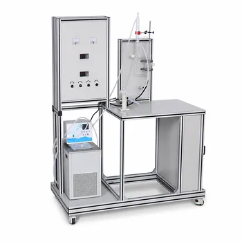
The core difference lies in the order of system dynamics. In a process control pilot plant, a single-tank liquid level system behaves as a first-order system, responding to a step change like a simple exponential lag. A double-tank (cascaded) system, however, introduces an additional energy storage element, transforming the response into a second-order characteristic with an initial delay and an S-shaped rise curve. Mathematically, this shifts the model from a first-order ordinary differential equation to a second-order one, directly impacting how you design and tune control loops.
A cascaded tank configuration eliminates the instant response seen in a single tank and replaces it with a smoother, delayed transient. The resulting second-order differential equation – characterized by two time constants and an overall gain – captures this multi-stage interaction, making the double-tank system an essential platform for teaching advanced control strategies like cascade control.
Why the Number of Tanks Changes Everything
The Single-Tank: A Textbook First-Order Lag
Applying a material balance to one tank with constant cross-sectional area (A) gives the classic first-order model.
The change in liquid volume equals inlet flow (Q_1) minus outlet flow (Q_2):
(\displaystyle A\frac{dh}{dt} = Q_1 - Q_2).
Assuming a linear outlet resistance (R_s) ((Q_2 = h / R_s)), the dynamics reduce to:
(\displaystyle T\frac{dh}{dt} + h = K Q_1),
where (T = A R_s) (time constant) and (K = R_s) (static gain).
The response to a step change in (Q_1) is immediate at (t=0) and moves exponentially toward the new steady state.
There is no overshoot, no inflection point – just a clean, predictable first-order lag.
This simplicity makes the single-tank ideal for introducing PID tuning and basic stability concepts.
The Double-Tank: Cascaded Storage Creates a Second-Order Response
When two tanks are connected in series, the intermediate flow (Q_{12}) becomes a function of the first tank’s level, and that flow then drives the second tank.
This “lag of a lag” fundamentally shifts the dynamic order.
For Tank 1: (A_1\frac{dh_1}{dt} = Q_1 - Q_{12}) with (Q_{12} = h_1 / R_1).
For Tank 2: (A_2\frac{dh_2}{dt} = Q_{12} - Q_2) with (Q_2 = h_2 / R_2).
Eliminating the intermediate variable (h_1) yields the governing second-order differential equation for the second tank’s level (h_2):
(\displaystyle T_1 T_2 \frac{d^2h_2}{dt^2} + (T_1 + T_2)\frac{dh_2}{dt} + h_2 = K Q_1).
Here, (T_1 = A_1 R_1) and (T_2 = A_2 R_2) are the individual time constants, and (K) is the overall system gain.
The open-loop step response now exhibits an S-shaped curve: a slow start (while the first tank fills), an inflection point where the rate of rise peaks, and then a gradual approach to steady state.
There is still no overshoot in a purely open-loop system, but the initial delay is stark.
Visualizing the Difference in the Control Room
A simple step test in your pilot plant tells the full story.
The single-tank trend immediately rises with its steepest slope at (t=0).
The double-tank trend lies nearly flat initially, then accelerates, and finally decelerates – a signature of overdamped second-order behavior.
This extra phase lag makes a P-only controller more prone to oscillation if not detuned, and it creates the perfect scenario for exploring cascade strategies that stabilize the first tank’s level as a secondary loop.
Understanding the Trade-offs
Added Realism vs. Experimental Complexity
A double-tank system more closely mimics many industrial series processes – distillation columns, cascaded reactors, heat exchangers in series – making it a superior model for process dynamics education.
However, the second-order nature means you must identify two time constants and a gain, complicating system identification exercises.
In a teaching lab, this can either be a powerful learning opportunity or a source of frustration if the fundamentals are not yet solid.
Sensitivity to Non-Ideal Valve Behavior
Both models assume the outlet valve resistance is linear and constant.
In real pilot plants, valve characteristics are notoriously nonlinear, and the effective resistance changes with flow.
This can distort the theoretical S-shaped response, introducing offsets or varying time constants.
Additionally, assumptions like perfect mixing and no interaction (backflow) are never fully met, creating teaching moments about model mismatch, but also demanding careful sensor and actuator selection.
Why Second-Order Opens the Door to Cascade Control
The primary control challenge in the double-tank case is the sluggish response of (h_2) to a change in (Q_1).
Cascade control masterfully addresses this: a fast secondary controller regulates (h_1) (or (Q_{12})) based on a setpoint provided by the primary controller that monitors (h_2).
This arrangement effectively compensates for the first tank’s lag, restoring a tighter overall response.
The double-tank rig is therefore not just a plant – it’s a live demonstration of why cascade structures exist.
Making the Right Choice for Your Goal
The choice between a single-tank and a double-tank system should be driven by your educational or research objectives, not by hardware availability alone.
- If your primary focus is teaching the fundamentals of feedback control and PID tuning: Start with the single-tank. Its clean first-order dynamics let students grasp time constants, gain, and loop stability without distraction.
- If your primary focus is demonstrating interaction, process delays, and advanced control strategies: Use the double-tank system. It directly illustrates the need for cascade control and provides rich data for second-order model identification.
- If your primary focus is simulating real industrial units in a pilot plant: The double-tank configuration is mandatory. It builds the intuition required for handling multi-capacity processes where successive lags demand structured controller hierarchies.
- If your primary focus is studying nonlinearity and model mismatch: A double-tank rig with variable position valves lets you explore how real nonlinearities deviate from the linear ODE, reinforcing the limits of textbook models.
Whichever configuration you choose, both systems are foundational building blocks. The key is to align the dynamic complexity with the specific control principle you want to illuminate – and the double-tank system, with its elegant second-order behavior, will always be your go-to for bridging fundamentals and industrial reality.
Summary Table:
| Feature | Single-Tank System | Double-Tank (Cascaded) System |
|---|---|---|
| System Order | First-order | Second-order |
| Response Type | Exponential lag (immediate rise at $t=0$) | S-shaped curve (delayed start & inflection) |
| Mathematical Model | $T \frac{dh}{dt} + h = K Q_1$ | $T_1 T_2 \frac{d^2h_2}{dt^2} + (T_1 + T_2)\frac{dh_2}{dt} + h_2 = K Q_1$ |
| Best Used For | Basic PID tuning & loop stability | Cascade control & model mismatch studies |
Bring Industrial-Scale Process Control into Your Lab
LABPARK designs and manufactures premium Educational and Vocational Unit Operations Pilot Plants in chemical engineering, bioprocess & biotech, and environmental & water treatment. Our state-of-the-art training rigs—including custom single and double-tank liquid level systems—equip universities, research institutes, and enterprises with the hands-on platforms needed to teach advanced process control and cascade loop configurations effectively.
Ready to elevate your engineering curriculum or research capabilities? Contact LABPARK today to customize your pilot plant setup.
Related Products
- Binary System Vapor Liquid Equilibrium Data Determination Educational Unit Operations Pilot Plant
- Ternary Liquid-Liquid Equilibrium Educational Pilot Plant
- Bench Scale Dual Column Gas Separation and Capture Educational Pilot Plant
- Two Phase Flow Pattern Velocity Resistance Measurement Educational Pilot Plant
- Two-Dimensional Fluidization Hydrodynamics Educational Pilot Plant for Unit Operations Training
People Also Ask
- Why correlate VLE pilot plant data using Wilson, NRTL, and UNIQUAC? Achieve Accurate Column Scale-Up
- For VLE Experiments: Fugacity vs. Activity Coefficient Method Selection Criteria
- How do pilot plants assist in teaching & researching non-ideal VLE? Bridge Theory & Physical Validation
- How to Model VLE for Supercritical & Unstable Components? Pilot Plant Methods
- Why is accurate VLE data critical? Optimize Unit Operations & Process Scale-Up