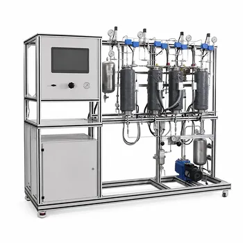
How To Show Constant Vs. Falling-Rate Drying? Guide To Unit Operations Pilot Plants.

Nothing cements theoretical kinetics like a real drying curve. By guiding students through a simple batch drying experiment in a pilot-scale unit operations plant, instructors transform abstract textbook equations into a story students can see. Students weigh the wet material at regular intervals, compute the moisture content, and then plot a drying rate curve. The moment the curve shifts from a flat plateau to a steep decline, the constant-rate and falling-rate drying periods become physically unmistakable.

The most effective way to demonstrate the difference is to have students collect weight‑vs‑time data under tightly controlled drying conditions and derive the drying rate curve. That curve’s shape—a horizontal line that suddenly plunges downward—is the fingerprint of the transition from surface‑controlled evaporation to diffusion‑limited internal moisture transport. The experiment makes the critical moisture content ((X_c)) a tangible, measurable design parameter rather than a fuzzy concept.

From Theory to a Visual Signature: Designing the Experiment

The core of the demonstration is a batch drying run performed under steady external conditions. A unit operations pilot plant is ideal because it gives students the hands‑on control and measurement resolution that desktop simulations simply cannot match.

Step 1: Running the Batch Drying Run

Instructors first help students lock in constant drying conditions—stable air temperature, humidity, and velocity—throughout the run. The wet material (often a granular solid or a filter cake) is loaded into the dryer, and the pilot plant’s instrumentation maintains these set‑points. Students record the weight of the wet material at uniform time intervals, capturing the gradual loss of moisture.

Step 2: Transforming Data into the Drying Rate Curve

From the weight data, students calculate the moisture content on a dry basis ((X)). They then derive the drying rate using a form of the rate equation seen in many lab manuals:

[ U = -\frac{G'}{S} \frac{dX}{d\tau} ]

(where (G') is the bone‑dry mass and (S) is the drying area). Plotting this drying rate against (X) yields a curve with two distinct regimes: a horizontal segment where the rate is constant, followed by a segment where the rate falls steadily as (X) decreases.

Step 3: Identifying the Critical Moisture Content ((X_c))

The sharp elbow where the plateau breaks marks the critical moisture content. Students can read (X_c) directly from the graph. This single parameter dictates how much drying time is spent in each regime and becomes the anchor for industrial dryer design calculations.

Understanding the Physics Behind the Curve

The visual story is only half the lesson. The real value lies in connecting each segment to the underlying transport mechanisms—and the pilot plant provides the data to do just that.

The Constant-Rate Period: Heat Transfer Governs

During this initial phase, the solid’s surface remains saturated with liquid. The drying rate is governed by external heat and mass transfer. If the pilot plant allows temperature monitoring (a thermocouple in the wet cake or at the surface), students will see that the material temperature stays steady at the wet‑bulb temperature of the drying air (or at the solvent’s boiling point if operating under vacuum). The drying rate can be modeled with a simple mass‑transfer equation, such as the one given in the primary reference for a specific system:

[ -\frac{dX}{d\tau} = 30,(H_{as} - H) ]

The physical takeaway is clear: as long as the surface stays wet, the rate depends only on air temperature, humidity, and velocity—not on the internal structure of the solid.

The Falling-Rate Period: Mass Transfer Takes Over

Once the moisture content drops below (X_c), the surface is no longer fully wetted. Internal diffusion becomes the bottleneck. The drying rate falls, and students can verify that increasing the air temperature now yields sharply diminishing returns. If temperature probes are placed in the material, they’ll observe the cake temperature beginning to rise, trending toward the heating jacket or bulk air temperature. The falling‑rate kinetics for many materials can be approximated by a linear relationship like:

[ -\frac{dX}{d\tau} = 1.2,X ]

This linear form reinforces that the process is controlled by the slow, tortuous journey of moisture from the interior to the surface.

Common Pitfalls to Avoid

Even a well‑designed pilot plant experiment can mislead if critical details are overlooked.

Unstable ambient conditions: Fluctuations in inlet air temperature or humidity directly distort the constant‑rate plateau. Students must monitor and log these parameters continuously.
Inadequate sampling frequency: Irregular or too‑infrequent weighings can mask the sharpness of the transition. Using an automated data‑logging balance eliminates guesswork.
Neglecting material variability: Non‑uniform initial moisture distribution or channeling in the bed can produce a smeared curve. Pre‑conditioning the material and loading it consistently are essential.
Oversimplifying the model: The constant‑ and falling‑rate equations provided are examples for specific systems. Students should understand that the underlying principles (heat‑transfer control vs. diffusion control) are universal, even if the exact coefficients vary.

Tailoring the Lab to Your Learning Objectives

A single experiment can be tuned to emphasize different concepts, depending on your curriculum.

If your primary focus is on dryer design and scale‑up: Center the analysis on determining (X_c) and using it to calculate total drying time. Have students compare different materials or conditions to see how (X_c) shifts.
If your primary focus is on heat and mass transfer fundamentals: Instrument the plant to record material temperature and exhaust humidity in parallel. Students then explain why the temperature is flat in the constant‑rate period and rises only after (X_c)—a direct demonstration of the shift from heat‑ to mass‑transfer control.
If your primary focus is on data analysis and process modeling: Challenge students to fit empirical equations to each region (e.g., constant‑rate linear model, falling‑rate power‑law model) and quantify deviations. Discuss the limitations of simplified models when extrapolating to different scales.

A single afternoon in the pilot plant gives your students a visual, quantitative, and physically intuitive understanding of drying kinetics that no textbook alone can deliver.

Summary Table:

Feature	Constant-Rate Period	Falling-Rate Period
Governing Mechanism	External heat & mass transfer	Internal moisture diffusion
Surface Saturated?	Yes (fully wet surface)	No (dry patches appear)
Material Temp.	Constant (at wet-bulb temp.)	Rising (approaching air temp.)
Key Rate Driver	Drying air velocity & humidity	Solid structure & internal diffusion

Bring abstract drying kinetics to life in your engineering labs. LABPARK provides premium Educational and Vocational Unit Operations Pilot Plants in chemical engineering, bioprocess & biotech, and environmental & water treatment for universities, research institutes, and enterprises. Our plants deliver the precise control and reliability needed to transform textbook theory into practical student mastery.

Ready to upgrade your laboratory capabilities? Contact us today to explore our custom solutions!