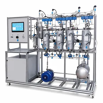
The main variable is the ultimate process condition you need to control—typically one that defines product quality or safety—while the secondary variable is a rapidly responding proxy that absorbs disturbances before they can corrupt that final outcome. On a chemical process control training unit, such as a reactor or heat exchanger pilot plant, the master controller monitors the main variable (e.g., reactor outlet temperature) and sets a dynamic setpoint for the secondary variable (e.g., jacket coolant flow). This architecture isolates fast-acting disturbances in the inner loop, shielding the primary process parameter from fluctuations and ensuring stable, precise control.
The main variable is your true process objective; the secondary variable is your first line of defense against disturbances. Their roles are distinct but interdependent, and their success hinges on a deliberate mismatch in their dynamic speeds—the secondary loop must be 3 to 10 times faster than the primary loop to avoid harmful oscillations.
Understanding the Role of the Primary (Main) Variable
The Main Variable as the Guardian of Quality
On any chemical pilot plant, the main variable is the process parameter that directly impacts safety, yield, or product specification. In a reactor, it is often the reaction temperature at the outlet; in a distillation column, it could be the overhead composition.
Its value determines whether the operation meets the desired quality standard. Any sustained deviation here translates directly into off-spec product or unsafe conditions.
The Master Controller Sets the Strategic Direction
The master controller receives the main variable measurement and compares it to the process setpoint. Its output is not sent to the final control element—instead, it becomes the remote setpoint for the secondary controller.
This hierarchical arrangement ensures that the slower, quality-defining variable governs the long-term control strategy, while the fast inner loop handles tactical disturbance rejection.
The Critical Role of the Secondary Variable
The Secondary Variable as a Fast-Acting Shield
The secondary variable is chosen for its sensitivity to upstream disturbances and its short response time. Common examples include jacket temperature, coolant flow rate, or steam pressure—anything that reacts almost instantly to process upsets.
When a disturbance hits (e.g., a sudden change in cooling water supply temperature), the secondary loop detects the deviation and corrects it before the main variable even notices. This shielding effect is the entire reason cascade control exists.
Dynamic Setpoint from the Master Controller
The slave controller does not operate on a fixed setpoint. It receives a continuously updated target from the master controller. This means the secondary variable is constantly re-tuned to serve the primary objective.
Think of it as an assistant that adjusts its own behavior in real time based on the boss’s latest instruction, never allowing short-term noise to distract from the long-term goal.
Why Dynamic Separation is Non-Negotiable
The 3-to-10 Ratio Rule
The primary and secondary processes have different time constants—the time it takes for them to respond significantly to a change. For stable cascade control, the secondary loop must be significantly faster.
The practical rule is that the primary time constant should be 3 to 10 times larger than the secondary time constant. This gap ensures the inner loop can settle a disturbance before its effect propagates to the outer loop.
Preventing Resonance Between the Loops
If the two time constants are too similar, the loops can begin to “talk” to each other in a destructive feedback cycle. The master controller adjusts the slave setpoint, the slave reacts, the master sees the result and adjusts again—all at a pace that creates oscillatory resonance.
The result is not just poor control; it can lead to a dangerously unstable process where temperature or pressure swings grow with each cycle.
Understanding the Trade-offs and Pitfalls
Risk of Instability from Mismatched Dynamics
Even a correctly architected cascade can fail if the process time constants drift due to fouling, load changes, or equipment wear. A secondary loop that becomes sluggish loses its shielding ability, while one that becomes too fast may overcorrect and overshoot.
On a training unit, deliberately mismatching these dynamics is a powerful way to demonstrate why the 3–10 ratio matters.
The Wrong Secondary Variable Can Undermine Control
Selecting a secondary variable that is not truly upstream of the primary disturbance—or that introduces its own noise—can degrade performance. For example, using a flow rate with excessive measurement lag as the secondary variable defeats the purpose of a fast inner loop.
The variable must be both fast and genuinely causal; otherwise, you are simply adding complexity without benefit.
How to Configure Your Training Unit for Success
The right variable pairing depends on what you want to teach or validate on the pilot plant.
- If your primary focus is product quality control: Choose the final reactor outlet temperature as the main variable and jacket inlet temperature as the secondary variable, ensuring the coolant loop responds at least 3 times faster than the reactor.
- If your primary focus is demonstrating disturbance rejection: Deliberately introduce an upstream disturbance (e.g., cooling water temperature dip) and confirm that a properly chosen secondary variable absorbs the upset before the main variable deviates significantly.
- If your primary focus is showing the limits of cascade control: Operate the unit with a time constant ratio near or below 2 to illustrate the dangerous oscillations that arise when loops are too closely coupled.
A cascade control system is only as effective as the dynamic separation between its loops—choose your variables to protect the main objective, not just to make an inner loop work faster.
Summary Table:
| Feature | Primary (Main) Variable | Secondary Variable |
|---|---|---|
| Core Objective | Controls final product quality & safety | Absorbs disturbances before they reach the main loop |
| Response Speed | Slower (Time constant is 3 to 10x larger) | Faster (Reacts almost instantly to changes) |
| Setpoint Source | User-defined target (Process operator) | Dynamically set by the master controller's output |
| Common Examples | Reactor outlet temperature, column composition | Jacket coolant flow, steam pressure, inlet temperature |
Elevate Your Chemical Engineering Lab with LABPARK
Ready to provide hands-on training with advanced process control? LABPARK designs and manufactures premium Educational and Vocational Unit Operations Pilot Plants in chemical engineering, bioprocess & biotech, and environmental & water treatment. We help universities, research institutes, and enterprises bridge the gap between theory and industrial practice with robust, real-world training systems.
Contact LABPARK today to discover how our pilot plants can enhance your curriculum and research capabilities!
Related Products
- Multi Pump Fluid Transport Process Piping Unit Operations Training Pilot Plant
- Chemical Pipeline Assembly and Fluid Transport Practical Training Unit Operations Pilot Plant
- Electrolyte Distillation Purification and Formulation Educational Pilot Plant
- Natural Product Extraction Unit Operations Training Pilot Plant
- Multi-Modal Distillation Unit Operations Training Pilot Plant
People Also Ask
- Why distinguish Newtonian & non-Newtonian fluids in pilot plants? Prevent design errors.
- Why is the chemical plant startup schedule crucial? De-risk scale-up with pilot plants.
- When to transition from PID to adaptive control in pilot plants? Key process indicators.
- How do deviations in estimating latent heat impact pilot plant thermal systems? Avoid hardware mis-sizing.
- Why Compare Predicted and Experimental Excess Enthalpy? Key to Accurate Pilot Plant Scale-up