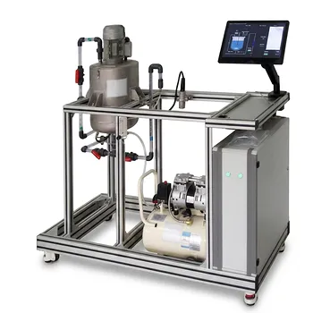
Here's the direct answer: Electrokinetic Instability (EKI) mixers use fluctuating electric fields—typically a sinusoidal AC signal—to drive oscillating electroosmotic flows. These flows relentlessly stretch and fold fluid interfaces, mimicking mechanical stirring without moving parts, and enable complete mixing in as little as 2.5 seconds at very low Reynolds numbers (~1). In lab-scale unit operations, this gives students a vivid, hands-on way to watch chaotic advection and micro-scale transport in real time.
EKI mixing turns a simple electric field into a virtual stir bar for the microscale. It lets teaching labs demonstrate how engineered chaos can overcome the otherwise slow, diffusion-limited mixing that plagues microfluidic devices—all with a visually compelling experiment that requires no fragile moving components.
How EKI Mixers Work: The Physics of Chaotic Flow
The core principle is generating unstable, time-dependent electroosmotic slip across the fluid domain. Instead of a steady DC field that would simply push fluid along in orderly streamlines, an AC field introduces constant disturbance and reorientation of the local flow.
The Role of Electroosmosis
EKI mixers begin with the same foundation as all electroosmotic flow.
When an electric field is applied parallel to a charged surface (like a microchannel wall), the mobile counter‑ions in the electrical double layer migrate, dragging the bulk fluid with them.
However, in a classic DC electroosmotic flow, the velocity profile is nearly plug‑like.
Mixing then relies solely on molecular diffusion, which is excruciatingly slow at the microscale.
Instability Through Fluctuating Fields
By applying a sinusoidal or alternating electric field, the flow is never allowed to reach a steady state.
The direction and magnitude of the electroosmotic slip velocity constantly change.
This continuous perturbation forces fluid elements on neighboring streamlines to diverge.
Any small concentration or conductivity gradient in the fluid gets amplified by the time‑dependent electric body force, triggering a hydrodynamic instability.
Stretching and Folding for Rapid Mixing
The instability manifests as a chaotic stretching‑and‑folding action at fluid interfaces.
Think of it as repeatedly kneading dough—the interface between two fluids is elongated exponentially, while folds bring layers close together.
This drastically increases the interfacial area across which diffusion can act.
Because the process is chaotic (sensitive to initial conditions), tiny, unpredictable flow structures emerge, distributing fluid parcels throughout the entire channel volume.
Performance Characteristics in Lab Demonstrations
The numbers that matter most for teaching unit operations are mixing time, Reynolds number, and visual clarity.
Mixing Time and Reynolds Number
At a flow Reynolds number of approximately 1, inertial mixing is essentially non‑existent.
EKI mixing forces the transition to a chaotic regime, achieving homogenization in roughly 2.5 seconds.
This is a dramatic demonstration point: without the field, the same fluids might take minutes or hours to mix via diffusion alone.
The experiment thus clearly isolates the contribution of advective flux, showing students that “flow” is more than just bulk velocity—it’s about how you stretch and redistribute concentration fields.
Visualization of Advective Flux
In a teaching lab, EKI mixers are often fabricated with transparent microchannels and observed under a microscope.
The use of fluorescent dyes or pH‑sensitive indicators makes the stretching‑and‑folding patterns directly visible.
Students can trace the evolution of chaotic streamlines, identifying the formation of whorls and tendrils.
This turns an abstract concept like “chaotic advection” into a tangible, easy‑to‑record phenomenon, reinforcing theoretical concepts from transport phenomena lectures.
Understanding the Trade-offs
For all its elegance, an EKI demonstration does come with constraints that instructors should anticipate.
Practical Constraints in a Teaching Lab
Generating the required fluctuating fields demands a high‑voltage AC source and careful electrode placement.
If the voltage is too low, the instability never kicks in and mixing remains diffusion‑dominated.
Electrode fouling or bubble generation (electrolysis) can also occur at the fluid‑electrode interface if the frequency or buffer conditions are not optimized.
These side effects may cloud the visual demonstration and require regular maintenance between lab sessions.
What EKI Demonstrations Do Not Show
The classic EKI mixer is most effective near Reynolds numbers around 1; it does not directly illustrate inertial turbulence.
Students must recognize that the chaotic patterns they see are electrically driven, not shear‑driven, which is a different paradigm from stirred‑tank mixing.
Additionally, the rapid mixing time is measured under well‑controlled microfluidic conditions.
Scaling the exact same physics to larger industrial mixers is not straightforward, so the demo serves best as a micro‑scale transport lesson, not a generic “mixing” blueprint.
Applying EKI in Your Curriculum
The ideal use of an EKI mixer depends on what you want students to take away from the lab.
- If your primary focus is showing that mixing is possible without moving parts: Demonstrate the dramatic difference between diffusion‑only and field‑assisted mixing side by side. Emphasize the 2.5‑second mixing time as a vivid performance benchmark.
- If your primary focus is teaching chaotic advection and fluid kinematics: Have students record video, trace fluid elements, and calculate Lyapunov exponents from the observed stretching rates. Frame the EKI mixer as a physical analog of the baker’s transformation.
- If your primary focus is connecting theory to transport equations: Guide students to identify the advective term in the species conservation equation and relate flow structures to the Péclet number. The EKI demo becomes a living example of how advective flux dominates when diffusion alone falls short.
A well‑run EKI mixing demo transforms a seemingly niche microfluidic phenomenon into a clear, reproducible lesson in transport fundamentals—arming students with a visceral understanding of flow, chaos, and the power of active mixing.
Summary Table:
| Feature | Operating Details | Educational Significance |
|---|---|---|
| Driving Force | Fluctuating AC electric fields | Demonstrates electric-field-driven active mixing |
| Mixing Mechanism | Chaotic stretching and folding | Physical model of chaotic advection & transport |
| Mixing Time | ~2.5 seconds (at Re ≈ 1) | Highlights advective flux over slow diffusion |
| Flow Regime | Low Reynolds number (~1) | Visualizes micro-scale fluid dynamics |
Bring Advanced Fluid Dynamics to Your Lab
Looking to upgrade your engineering curriculum or research capabilities? LABPARK provides state-of-the-art Educational and Vocational Unit Operations Pilot Plants in chemical engineering, bioprocess & biotech, and environmental & water treatment. We help universities, research institutes, and enterprises bridge the gap between theory and hands-on practice with reliable, high-performance training equipment.
Contact LABPARK today to discover how our pilot plants can enhance your teaching and research outcomes!
Related Products
People Also Ask
- How do cost-capacity exponents vary across chemical equipment? Scaling insights.
- What are the primary considerations when managing and scaling up shear rates in pilot plant mixing operations? Guide
- What are the differences between set-point, servo, and program control? Master unit operations training.
- Evaluate Tablet Compaction: Force, Density & Porosity in Unit Operations Pilot Plants
- Why Switch Unit Operations Flow Configurations? Impact on Experimental Measurements